Calculating tolerance limits — such as A-Basis and B-Basis is an important part of developing and certifying composite structure for aircraft. When the data doesn’t fit a convenient parametric distribution like a Normal or Weibull distribution, one often resorts to non-parametric methods. Several non-parametric methods exist for determining tolerance limits.
Vangel’s 1994 paper Vangel (1994) discusses a non-parametric method for determining tolerance limits. This article provides a brief summary of that work and discusses the implementation of that method in the R language, as well as some choices that can be made in the implementation.
This method of calculating non-parametric tolerance limits is an extension of the Hanson—Koopmans method Hanson and Koopmans (1964) . The lower tolerance can be calculated using the following formula:
where \(x_{(i)}\) and \(x_{(j)}\) indicate the \(i\)th and \(j\)th order statistic of the sample (that is, the \(i\)th smallest and the \(j\)th smallest value).
The values of \(j\) and \(z\) need to be determined somehow.
There is a function \(H(z)\) defined as follows:
where \(\beta\) is the content of the desired tolerance limit. The details are outside the scope of this article, but we can write a function that solves the following equation for \(z\).
where \(\gamma\) is the confidence of the desired tolerance limit.
It turns out that we obtain different values of \(z\) depending on which values of \(i\) and \(j\) we choose.
Vangel’s approach is to set \(i=1\) in all cases, then to find the value of \(j\) that would produce a tolerance limit that is nearest to the population quantile assuming that the data is distributed according to a standard normal distribution.
We’ll investigate this approach through simulation. First, we’ll load a few packages.
library(tidyverse)
library(cmstatr)
Next, we’ll set the value of \(i=1\) and a value of the content and confidence of our tolerance limit. We’ll choose B-Basis tolerance limits as an example.
i <- 1
p <- 0.90
conf <- 0.95
The expected value of the \(i\)th order statistic for a normally distributed sample can be calculated using the following function (see Harter (1961) ). We’ll need this function soon.
expected_order_statistic <- function(i, n) {
  int <- function(x) {
    x * pnorm(-x) ^ (i - 1) * pnorm(x) ^ (n - i) * dnorm(x)
  }
  integral <- integrate(int, -Inf, Inf)
  stopifnot(integral$message == "OK")
  factorial(n) / (factorial(n - i) * factorial(i - 1)) * integral$value
}
When using Vangel’s approach, we need to minimize the value of the following function.
fcn <- function(j, n) {
  e1 <- expected_order_statistic(i, n)
  e2 <- expected_order_statistic(j, n)
  z <- hk_ext_z(n, i, j, p, conf)
  abs(z * e1 + (1 - z) * e2 - qnorm(p))
}
We can plot the above function versus \(j\) for the value of \(n=17\):
data.frame(
  j = seq(7, 11, by = 0.1)
) %>%
  mutate(fcn = Vectorize(fcn)(j, 17)) %>%
  ggplot(aes(x = j, y = fcn)) +
  geom_line() +
  geom_point(
    data = data.frame(j = 7:11) %>%
      mutate(fcn = Vectorize(fcn)(j, 17)),
    mapping = aes(x = j, y = fcn)
  )
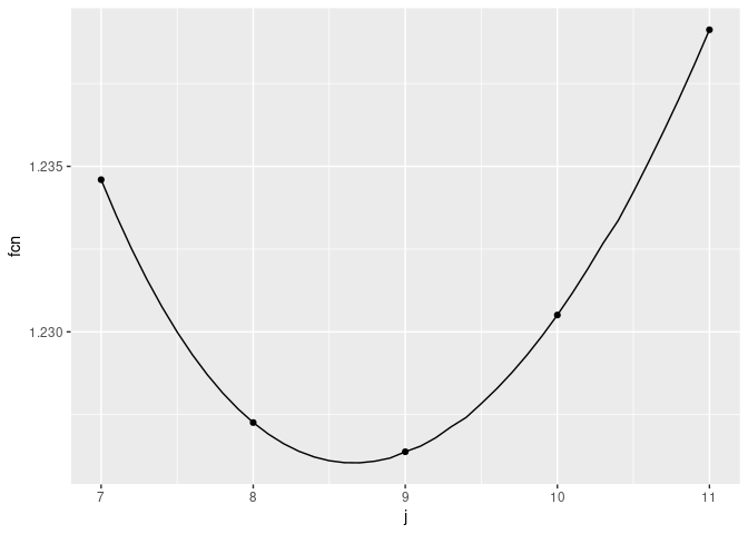
In this particular case, we can see that \(j=9\) produces the minimum value of this function (for integer values of \(j\)). But this function at \(j=8\) is not much worse.
Of note, there is a table of optimum values of \(j\) for various values of \(n\) published in CMH-17-1G [@CMH-17-1G] 1. For most values of \(n\), the optimum value from the function above matches the published value. However, for samples of size 17, 20, 23, 24 and 28, the function above disagrees with the published values by one unit. We will focus the simulation effort on samples of these sizes. For sample sizes of interest, the following values of \(j\) and \(z\) are published in CMH-17-1G.
published_r_n <- tribble(
  ~n, ~j_pub, ~z_pub,
  17, 8, 1.434,
  20, 10, 1.253,
  23, 11, 1.143,
  24, 11, 1.114,
  28, 12, 1.010
)
We can create an R function that returns the “optimum” value of \(j\) where all the integer values of \(j\) are considered, then the integer with the lowest value of that function is returned. Such an R function is as follows:
optim_j <- function(n) {
  j <- 2:n
  f <- sapply(2:n, function(j) Vectorize(fcn)(j, n))
  j[f == min(f)]
}
For values of \(n\) of interest, we’ll generate a large number of samples (10,000) drawn from a normal distribution. We can calculate the true population quantile, since we know the population parameters. We can use the two variations of the nonparametric tolerance limit approach to calculate tolerance limits. The proportion of those tolerance limits that are below the population quantile should equal the selected confidence level. We’ll restrict the simulation to values of \(n\) where we find different values of \(j\) compared with those publised in CMH-17-1G.
mu_normal <- 100
sd_normal <- 6

set.seed(1234567)  # make this reproducible

sim_normal <- pmap_dfr(published_r_n, function(n, j_pub, z_pub) {
  j_opt <- optim_j(n)
  z_opt <- hk_ext_z(n, i, j_opt, p, conf)

  map_dfr(1:10000, function(i_sim) {
    tibble(
      n = n,
      x = list(sort(rnorm(n, mu_normal, sd_normal))),
      j_pub = j_pub,
      j_opt = j_opt,
      z_pub = z_pub,
      z_opt = z_opt,
    )
  }
  )
}) %>%
  rowwise() %>%
  mutate(
    T_pub = x[j_pub] * (x[i] / x[j_pub]) ^ z_pub,
    T_opt = x[j_opt] * (x[i] / x[j_opt]) ^ z_opt
  )
sim_normal
## # A tibble: 50,000 × 8
## # Rowwise:
##        n x          j_pub j_opt z_pub z_opt T_pub T_opt
##    <dbl> <list>     <dbl> <int> <dbl> <dbl> <dbl> <dbl>
##  1    17 <dbl [17]>     8     9  1.43  1.40  85.4  85.4
##  2    17 <dbl [17]>     8     9  1.43  1.40  89.5  89.3
##  3    17 <dbl [17]>     8     9  1.43  1.40  83.2  83.5
##  4    17 <dbl [17]>     8     9  1.43  1.40  83.6  83.8
##  5    17 <dbl [17]>     8     9  1.43  1.40  83.4  83.8
##  6    17 <dbl [17]>     8     9  1.43  1.40  84.1  84.4
##  7    17 <dbl [17]>     8     9  1.43  1.40  82.6  82.9
##  8    17 <dbl [17]>     8     9  1.43  1.40  87.5  87.6
##  9    17 <dbl [17]>     8     9  1.43  1.40  83.9  83.8
## 10    17 <dbl [17]>     8     9  1.43  1.40  86.9  87.2
## # … with 49,990 more rows
We can plot the distribution of the tolerance limits that result from our R code and from the values of \(j\) and \(z\) published in CMH-17-1G. We see that the distributions are very similar.
sim_normal %>%
  pivot_longer(cols = T_pub:T_opt, names_to = "Approach") %>%
  ggplot(aes(x = value, color = Approach)) +
  geom_density() +
  facet_wrap(n ~ .) +
  ggtitle("Distribution of Tolerance Limits for Various Values of n")
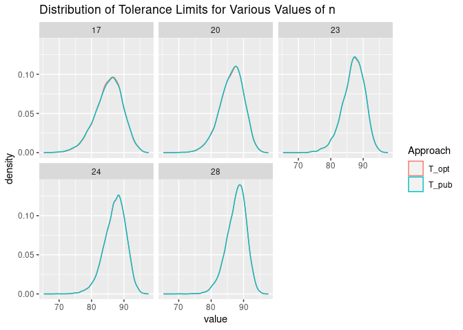
In this article, we’re calculating the B-Basis (lower 90/95 tolerance limit). So, the population quantile that we’re approximating is:
x_p_normal <- qnorm(1 - p, mu_normal, sd_normal)
x_p_normal
## [1] 92.31069
We can now determine what proportion of the calculated tolerance limits were below the population quantile.
sim_normal %>%
  mutate(below_pub = T_pub < x_p_normal,
         below_opt = T_opt < x_p_normal) %>%
  group_by(n) %>%
  summarise(
    prop_below_pub = sum(below_pub) / n(),
    prop_below_opt = sum(below_opt) / n()
  )
## # A tibble: 5 × 3
##       n prop_below_pub prop_below_opt
##   <dbl>          <dbl>          <dbl>
## 1    17          0.964          0.967
## 2    20          0.967          0.965
## 3    23          0.960          0.960
## 4    24          0.959          0.957
## 5    28          0.954          0.954
In all cases, the tolerance limits are conservative when the data are normally distributed. Remember that we expect that 95% of the tolerance limits should be below the population quantile: here we see a slightly higher proportion than 95%.
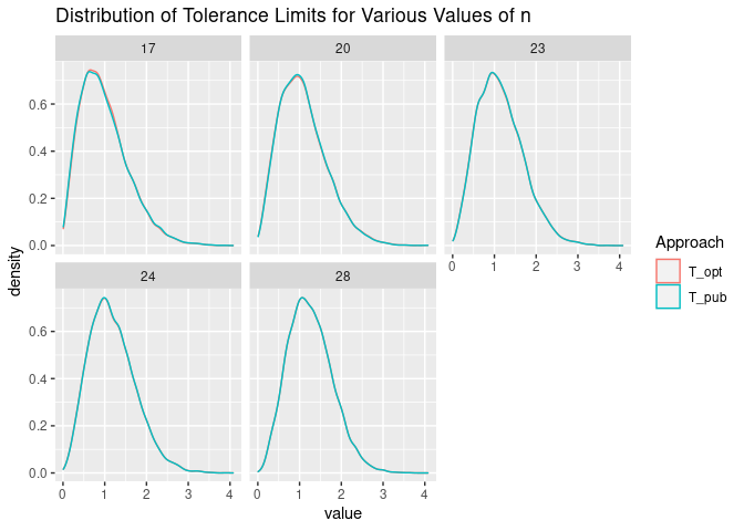
We can repeat this with a distribution that is far from normal. Let’s try it withe the \(\chi^2\) distribution.
df_chisq <- 6

set.seed(2345678)  # make this reproducible

sim_chisq <- pmap_dfr(published_r_n, function(n, j_pub, z_pub) {
  j_opt <- optim_j(n)
  z_opt <- hk_ext_z(n, i, j_opt, p, conf)

  map_dfr(1:10000, function(i_sim) {
    tibble(
      n = n,
      x = list(sort(rchisq(n, df_chisq))),
      j_pub = j_pub,
      j_opt = j_opt,
      z_pub = z_pub,
      z_opt = z_opt,
    )
  }
  )
}) %>%
  rowwise() %>%
  mutate(
    T_pub = x[j_pub] * (x[i] / x[j_pub]) ^ z_pub,
    T_opt = x[j_opt] * (x[i] / x[j_opt]) ^ z_opt
  )
sim_chisq
## # A tibble: 50,000 × 8
## # Rowwise:
##        n x          j_pub j_opt z_pub z_opt T_pub T_opt
##    <dbl> <list>     <dbl> <int> <dbl> <dbl> <dbl> <dbl>
##  1    17 <dbl [17]>     8     9  1.43  1.40 1.00  1.03
##  2    17 <dbl [17]>     8     9  1.43  1.40 1.35  1.34
##  3    17 <dbl [17]>     8     9  1.43  1.40 1.39  1.40
##  4    17 <dbl [17]>     8     9  1.43  1.40 1.39  1.28
##  5    17 <dbl [17]>     8     9  1.43  1.40 1.39  1.43
##  6    17 <dbl [17]>     8     9  1.43  1.40 0.283 0.297
##  7    17 <dbl [17]>     8     9  1.43  1.40 0.514 0.497
##  8    17 <dbl [17]>     8     9  1.43  1.40 0.264 0.268
##  9    17 <dbl [17]>     8     9  1.43  1.40 1.68  1.61
## 10    17 <dbl [17]>     8     9  1.43  1.40 0.661 0.692
## # … with 49,990 more rows
The population quantile is:
x_p_chisq <- qchisq(1 - p, df_chisq)
x_p_chisq
## [1] 2.204131
The distribution of the tolerance limits calculated using the values of \(j\) and \(z\) that we calculate and those published. Again, the distributions are very similar.
sim_chisq %>%
  pivot_longer(cols = T_pub:T_opt, names_to = "Approach") %>%
  ggplot(aes(x = value, color = Approach)) +
  geom_density() +
  facet_wrap(n ~ .) +
  ggtitle("Distribution of Tolerance Limits for Various Values of n")
We can now determine what proportion of the calculated tolerance limits were below the population quantile.
sim_chisq %>%
  mutate(below_pub = T_pub < x_p_chisq,
         below_opt = T_opt < x_p_chisq) %>%
  group_by(n) %>%
  summarise(
    prop_below_pub = sum(below_pub) / n(),
    prop_below_opt = sum(below_opt) / n()
  )
## # A tibble: 5 × 3
##       n prop_below_pub prop_below_opt
##   <dbl>          <dbl>          <dbl>
## 1    17          0.963          0.965
## 2    20          0.959          0.959
## 3    23          0.959          0.958
## 4    24          0.955          0.955
## 5    28          0.953          0.953
Again with this distribution, we see that the tolerance limits are conservative.
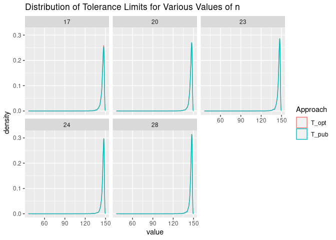
Finally, let’s try again using a t-Distribution.
df_t <- 3
offset_t <- 150

set.seed(4567)  # make this reproducible

sim_t <- pmap_dfr(published_r_n, function(n, j_pub, z_pub) {
  j_opt <- optim_j(n)
  z_opt <- hk_ext_z(n, i, j_opt, p, conf)

  map_dfr(1:10000, function(i_sim) {
    tibble(
      n = n,
      x = list(sort(rt(n, df_t) + offset_t)),
      j_pub = j_pub,
      j_opt = j_opt,
      z_pub = z_pub,
      z_opt = z_opt,
    )
  }
  )
}) %>%
  rowwise() %>%
  mutate(
    T_pub = x[j_pub] * (x[i] / x[j_pub]) ^ z_pub,
    T_opt = x[j_opt] * (x[i] / x[j_opt]) ^ z_opt
  )
sim_t
## # A tibble: 50,000 × 8
## # Rowwise:
##        n x          j_pub j_opt z_pub z_opt T_pub T_opt
##    <dbl> <list>     <dbl> <int> <dbl> <dbl> <dbl> <dbl>
##  1    17 <dbl [17]>     8     9  1.43  1.40  140.  140.
##  2    17 <dbl [17]>     8     9  1.43  1.40  147.  147.
##  3    17 <dbl [17]>     8     9  1.43  1.40  144.  144.
##  4    17 <dbl [17]>     8     9  1.43  1.40  147.  147.
##  5    17 <dbl [17]>     8     9  1.43  1.40  147.  147.
##  6    17 <dbl [17]>     8     9  1.43  1.40  145.  145.
##  7    17 <dbl [17]>     8     9  1.43  1.40  146.  146.
##  8    17 <dbl [17]>     8     9  1.43  1.40  147.  147.
##  9    17 <dbl [17]>     8     9  1.43  1.40  146.  146.
## 10    17 <dbl [17]>     8     9  1.43  1.40  143.  143.
## # … with 49,990 more rows
The population quantile is:
x_p_t <- qt(1 - p, df_t) + offset_t
x_p_t
## [1] 148.3623
The distribution of the tolerance limits using the two approaches are as follows. Again, the distributions are very similar.
sim_t %>%
  pivot_longer(cols = T_pub:T_opt, names_to = "Approach") %>%
  ggplot(aes(x = value, color = Approach)) +
  geom_density() +
  facet_wrap(n ~ .) +
  ggtitle("Distribution of Tolerance Limits for Various Values of n")
We can now determine what proportion of the calculated tolerance limits were below the population quantile.
sim_t %>%
  mutate(below_pub = T_pub < x_p_t,
         below_opt = T_opt < x_p_t) %>%
  group_by(n) %>%
  summarise(
    prop_below_pub = sum(below_pub) / n(),
    prop_below_opt = sum(below_opt) / n()
  )
## # A tibble: 5 × 3
##       n prop_below_pub prop_below_opt
##   <dbl>          <dbl>          <dbl>
## 1    17          0.958          0.959
## 2    20          0.953          0.952
## 3    23          0.953          0.953
## 4    24          0.954          0.954
## 5    28          0.953          0.953
For this distribution, the tolerance limits are still conservative.
From this simulation work, it appears that both approaches to selecting the value of \(j\) preform equally well. The tolerance limits produced using each approach for a particular sample will be different, but both approaches seem to be equally valid.
The R package cmstatr contains the function hk_ext_z_j_opt which
returns \(j\) and \(z\) for calculating tolerance limits with the
optimization method described here (after version 0.8.02). While the
tolerance limits found for some particular samples may differ slightly
from that produced by the tables published in CMH-17-1G, both results
appear are equally valid.
-
It should be noted that CMH-17-1G uses \(r\) and \(k\) instead of \(j\) and \(z\) as used in this article and in Vangel’s paper. ↩
-
cmstatrversion 0.8.0 and earlier used a slightly different function that was optimized. That version of the code produces slightly different values of \(j\) for certain values of \(n\). ↩
Citations
- Mark Vangel. One-sided nonparametric tolerance limits. Communications in Statistics - Simulation and Computation, 23(4):1137–1154, 1994. doi:10.1080/03610919408813222. 1
- D. L. Hanson and L. H. Koopmans. Tolerance limits for the class of distributions with increasing hazard rates. The Annals of Mathematical Statistics, 35(4):1561–1570, 1964. doi:10.1214/aoms/1177700380. 1
- H. Leon Harter. Expected values of normal norder statistics. Biometrika, 48(1/2):151–165, 1961. doi:https://doi.org/10.2307/2333139. 1