There are a lot of misconceptions about bonded joints. One of the misconceptions that I’ve seen most often is that people think that the average shear stress in a lap joint is predictive of the strength. This same misconception is usually phrased as either:

• Doubling the overlap length of a lap joint doubles the strength (wrong!)
• Calculate $P/A$ for the joint and make sure that the value is less than the lap shear strength on the adhesive data-sheet (wrong!)

In this post, I’m going to explain why these statements are incorrect. I’m going to try to give you a understanding of how load transfer works in an adhesive joint, and I’m going to share some Python code that produces a first approximation of the stress distribution.

For simplicity, we’re going to ignore the effects of peel. Peel is the tendency for the ends of a lap joint to separate. This can cause the joint to fail in some cases, but considering the effects of peel complicates the analysis of the joint — since the purpose of this post is to give a basic understanding of the mechanics of the joint, I’m going to ignore this complicating factor.

The Joint

In this post, I’m going to focus on a simple lap joint. In this type of joint, two adherends overlap each other by a certain amount and there is adhesive connecting the two adherends over the area in which they overlap. These two adherends are then pulled apart. In this post, we’re going to assume that the two adherends are homogeneous isotropic materials (for example, sheet metal) and are uniform thickness. This joint is shown in the figure below. In the top part of the figure, we see the unstressed joint, and in the bottom, we see the joint under load.

Obviously, the deformation of the joint is exaggerated, but it allows us to see what’s happening.

First, let’s look at the lower adherend. We see that the left edge of the adherend is built-in (i.e. it can’t move). When load is applied, the left portion of the lower adherend stretches a lot because it is carrying the entirety of the reaction load.

As we move our gaze further to the right, but still focusing on the lower adherend, we see that the further right we go, the less the adherend is stretching. This is because the adhesive is transferring load along the length of the joint. When we look at the right portion of the lower adherend, it’ hardly stretched at all. Sure, it moved because the rest of the adherend has stretched, but the right part of the lower adherend has hardly stretched at all since it’s carrying no load.

If the two adherends are the same thickness, then symmetry will tell us that the upper adherend behaves in the same way — but now is the right end of the upper adherend that stretches a lot and the left end that doesn’t stretch.

Now, let’s turn our attention to the adhesive. Shear strain can be though of as an angle. At the very left edge of adhesive, the shear strain is quite large, in the middle of the adhesive, the shear strain is moderate and at the right edge of the adhesive, the shear strain is quite large again. The relationship between shear stress and shear strain of an adhesive is not linear, but nonetheless, a large strain produces a large stress and a small strain produces a small stress. So, the shear stress distribution in this joint is “U” shaped — there’s a lot of stress at the ends and a smaller stress in the middle.

This “U” shaped shear stress distribution should be the first clue about why using the average shear stress in the joint to predict failure might not be the best idea.

A Linear Model of the Joint

The actual shear stress-shear strain relationship for most adhesives is non-linear, but we’ll start our analysis of a lap joint by making the assumption that the adhesive is linear-elastic.

Let’s start with defining the variables that we’ll need. The variables are shown in the following figure.

A force balance on the two adherends gives us:

$$ \frac{dN_1}{dx} - \tau = 0 $$

$$ \frac{dN_2}{dx} + \tau = 0 $$

We can find the deformation of the two adherends as follows:

$$ \frac{du_1}{dx} = \frac{N_1}{E_1^\prime t_1} $$

$$ \frac{du_2}{dx} = \frac{N_2}{E_2^\prime t_2} $$

Where $E_1^\prime$ and $E_2^\prime$ are the adherend plane-strain elastic moduli.

The shear strain of the adhesive layer is given by:

$$ \gamma = \frac{1}{t_A} \left(u_1 - u_2\right) $$

We can differentiate this with respect to $x$ and then substitute in the previous equations to get:

$$ \frac{d\gamma}{dx} = \frac{1}{t_A}\left( \frac{du_1}{dx} - \frac{du_2}{dx} \right) \ {} = \frac{1}{t_A}\left( \frac{N_1}{E_1^\prime t_1} - \frac{N_2}{E_2^\prime t_2} \right) $$

We can then differentiate this again with respect to $x$ and substituting in the first equations, we get:

$$ \frac{d^2\gamma}{dx^2} = \frac{1}{t_A}\left( \frac{dN_1}{dx}\frac{1}{E_1^\prime t_1} - \frac{dN_2}{dx}\frac{1}{E_2^\prime t_2} \right) \ {} = \tau\frac{1}{t_A}\left( \frac{1}{E_1^\prime t_1} + \frac{1}{E_2^\prime t_2} \right) $$

Remember that for now, we’re assuming that the adhesive is linear-elastic. Thus:

$$ \tau = G_A \gamma $$

We can solve the second-order differential equation above, but we need two boundary conditions. The boundary conditions that we choose are the loads at the ends of the adherends. At the left end ($x=0$), the unit load on the lower adherend ($N_2$) must be equal to the applied load ($P$) divided by the width ($w$) and the load on the upper adherend ($N_1$) must be zero. The opposite is true at the other end ($x=L$). Thus:

$$ \left.N_1\right|{x=0} = 0 \ \left.N_2\right| = P/w $$

$$ \left.N_1\right|{x=L} = P/w \ \left.N_2\right| = 0 $$

We can plug these into the equation for $\frac{d\gamma}{dx}$ at the two ends of the joint and get the following boundary conditions that we will enforce for the solution.

$$ \left.\frac{d\gamma}{dx}\right|_{x=0} = \frac{1}{t_A}\left( \frac{-P / w}{E_2^\prime t_2} \right) $$

$$ \left.\frac{d\gamma}{dx}\right|_{x=L} = \frac{1}{t_A}\left( \frac{P / w}{E_1^\prime t_1} \right) $$

There is a closed-form solution to this boundary value problem, which we could find, but I think it’s more instructive to just find a numerical solution — plus it’s easier to extend the numerical solution to the case where the adhesive is non-linear. In order to find the numerical solution, we’re going to use the Python package scipy, which includes the function solve_bvp() for solving boundary-value problems. We’ll start by importing the packages that we’ll use.

import numpy as np
import scipy.integrate
import matplotlib.pyplot as plt

Next, we’ll set the parameters for our solution. These include the elastic moduli, thicknesses, overlap length and load.

E1 = 10.5e6 / (1 - 0.33**2)
E2 = 10.5e6 / (1 - 0.33**2)
t1 = 0.063
t2 = 0.063
Ga = 65500
ta = 0.005

L = 0.5
w = 1.

P = 2700

The function solve_bvp requires two arguments: (i) a function that returns the derivatives of the variables, and (ii) a function that returns the residuals for the boundary conditions. We’re going to reduce the second-order differential equation to a system of two first-order differential equations by defining $y$ as follows. Based on this definition, we can implement the two functions required by solve_bvp.

$$ y = \left[ \begin{matrix} \frac{d\tau}{dx} & \tau \end{matrix} \right]^T $$

def func1(x, y):
  D = np.matrix([
    [0, Ga / ta * (1. / (E1 * t1) + 1. / (E2 * t2))],
    [1, 0]
  ])
  return D @ y

def bc1(ya, yb):
  return np.array([
    ya[0] - 1. / ta * (-P / w / (E2 * t2)),
    yb[0] - 1. / ta * (P / w / (E1 * t1))
  ])

res1 = scipy.integrate.solve_bvp(
  func1,
  bc1,
  x = np.linspace(0, L, num=50),
  y = np.zeros((2, 50))
)

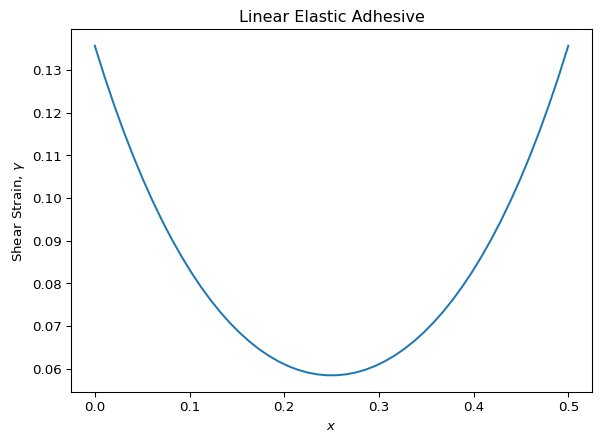
The variable res1 now contains the solution to our differential equation. We can plot the shear strain ($\gamma$) over the length of the joint as follows:

plt.plot(res1.x, res1.y[1,:])
plt.title("Linear Elastic Adhesive")
plt.ylabel("Shear Strain, $\\gamma$")
plt.xlabel("$x$")
plt.show()

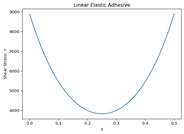
Because we’re assuming that the adhesive is linear-elastic, we can find the shear stress by simply multiplying the elastic modulus $G_A$ by the shear strain. The shear stress in the adhesive over the length of the joint is thus:

plt.plot(res1.x, Ga * res1.y[1,:])
plt.title("Linear Elastic Adhesive")
plt.ylabel("Shear Stress, $\\tau$")
plt.xlabel("$x$")
plt.show()

Stress-Strain Curve

The shear stress-strain curve for most adhesives is linear at low strain, but highly nonlinear above a certain value of strain. It’s common to idealize the stress-strain curve for an adhesive as elastic-perfectly plastic. The important parameters for the adhesive stress-strain curve are the initial shear modulus ($G_A$), the strain at yield ($\gamma_y$), from which you can calculate a shear stress at yield. The other important parameter is the ultimate strain, which we’ll talk about later. The idealized stress-strain curve therefore looks like this:

The ordinary approach to solving the stress distribution within a bonded joint involves finding the points along the length of the joint at which the adhesive transitions from elastic to plastic and then solving the elastic and plastic portions of the joint separately. If you try to naively solve the equations above with an elastic-perfectly plastic adhesive model, you’ll get errors since the Jacobian become singular. For the purpose of keeping this blog post simple, we’ll cheat a little bit and give the the stress-strain curve a very small slope above the yield stress. This will eliminate the numerical issues, and as as long as this slope is small enough, it won’t affect the results very much.

With this in mind, and considering that the strain could be positive or negative, we implement a function to find the stress based on the strain as follows:

def calc_tau(gamma):
  gamma_y = 0.09  # the yield strain
  G_final = 1  # a very small slope for the upper part of the curve
  sign = np.sign(gamma)
  if np.abs(gamma) <= gamma_y:
    tau_unsigned = Ga * np.abs(gamma)
  else:
    tau_unsigned = Ga * gamma_y + \
      G_final * (np.abs(gamma) - gamma_y)
  return sign * tau_unsigned

We’ll vectorize this function so that we can calculate an array of stress values based on an array of strain values:

calc_tau_vec = np.vectorize(calc_tau)

A Nonlinear Model of the Joint

Now that we have a function to describe the way in which the adhesive creates shear stress depending on its shear strain, we can implement the solution to the differential equation again. Since the boundary conditions don’t depend on the behavior of the adhesive, we can re-use the same function for calculating the residuals of the boundary condition.

def func2(x, y):
  b = (1. / (E1 * t1) + 1. / (E2 * t2)) / ta
  return np.row_stack((
    calc_tau_vec(y[1, :]) * b,
    y[0, :]
  ))


res2 = scipy.integrate.solve_bvp(
  func2,
  bc1,
  x = np.linspace(0, L, num=50),
  y = np.zeros((2, 50))
)

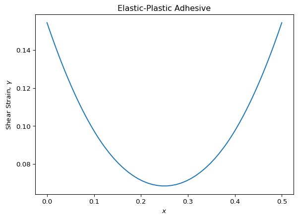
Here is the strain solution that we get:

plt.plot(res2.x, res2.y[1,:])
plt.title("Elastic-Plastic Adhesive")
plt.ylabel("Shear Strain, $\\gamma$")
plt.xlabel("$x$")
plt.show()

And the corresponding adhesive shear stress solution is as follows:

plt.plot(res2.x, calc_tau_vec(res2.y[1,:]))
plt.title("Elastic-Plastic Adhesive")
plt.ylabel("Shear Stress, $\\tau$")
plt.xlabel("$x$")
plt.show()

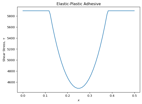
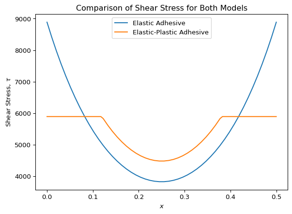
We’ll overlay the linear and the elastic-plastic models on top of each other to clearly show the differences between the two models. First, we notice that the elastic-plastic model has flat spots in the stress distribution where the adhesive has yielded. These occur near the ends of the joint. Next, we notice that the middle of the two stress distributions look similar, but shifted: for the elastic-plastic model, the stress in the “trough” is higher because the ends of this joint take a smaller proportion of the entire load.

plt.plot(res1.x, Ga * res1.y[1,:], label="Elastic Adhesive")
plt.plot(res2.x, calc_tau_vec(res2.y[1,:]), label="Elastic-Plastic Adhesive")
plt.title("Comparison of Shear Stress for Both Models")
plt.ylabel("Shear Stress, $\\tau$")
plt.xlabel("$x$")
plt.legend()
plt.show()

Exploration

We’ll create a function that takes several of the joint parameters as arguments and returns the stress and strain distributions. We’ll use this function to explore the effect of some of the joint parameters. We’re only going to implement this for the elastic-plastic model.

def model(t1, t2, ta, L, P):
  def ode(x, y):
    b = (1. / (E1 * t1) + 1. / (E2 * t2)) / ta
    return np.row_stack((
      calc_tau_vec(y[1, :]) * b,
      y[0, :]
    ))

  def bc(ya, yb):
    return np.array([
      ya[0] - 1. / ta * (-P / w / (E2 * t2)),
      yb[0] - 1. / ta * (P / w / (E1 * t1))
    ])

  res = scipy.integrate.solve_bvp(
    ode,
    bc,
    x = np.linspace(0, L, num=50),
    y = np.zeros((2, 50))
  )

  x = res.x
  gamma = res.y[1,:]
  tau = calc_tau_vec(gamma)

  return x, gamma, tau

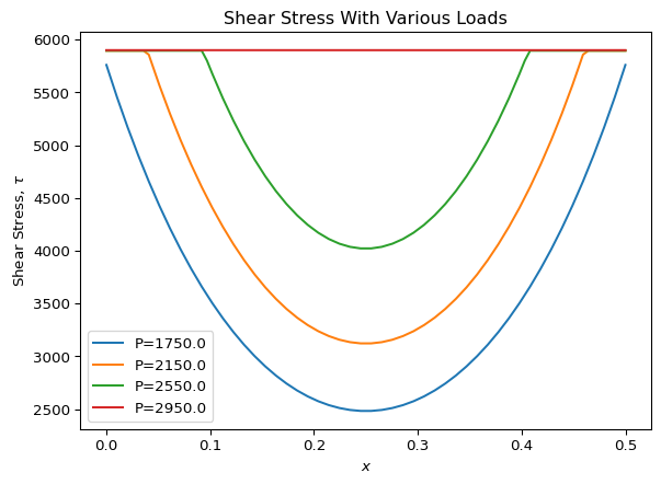
First, we’ll keep all of the parameters constant except that we’ll vary the load. This will show us how the stress distribution changes as we increase the load. The results aren’t surprising. At low loads, the joint is fully elastic. As the load is increased, the adhesive at the ends of the overlap start to yield. As load is increased further, the yielded area grows and the “trough” gets shallower. Finally, the joint becomes fully plastic. At this point, the joint would surely fail, but since our model doesn’t check for failure, we don’t see this.

for Pi in np.linspace(1750, 2950, num=4):
  x_i, gamma_i, tau_i = model(
    t1=t1, t2=t2, ta=ta, L=L, P=Pi
  )
  plt.plot(x_i, tau_i, label=f"P={Pi}")
plt.title("Shear Stress With Various Loads")
plt.ylabel("Shear Stress, $\\tau$")
plt.xlabel("$x$")
plt.legend()
plt.show()

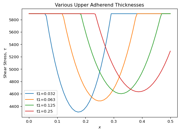
Next, we’ll see what happens when we change the thickness of the upper adherend. In this example, the lower adherend has a thickness of $t_2=0.063$ and we vary the thickness of the upper adherend ($t_1$) from half this thickness to four times this thickness. As we can see, this changes the length of the two plastic zones: in the extreme case of $t_1=0.250$, there is no plastic zone on the right because the adherend carrying the load at the right end of the joint is so stiff.

for t1_i in [0.032, 0.063, .125, .250]:
  x_i, gamma_i, tau_i = model(
    t1=t1_i, t2=t2, ta=ta, L=L, P=P
  )
  plt.plot(x_i, tau_i, label=f"t1={t1_i}")
plt.title("Various Upper Adherend Thicknesses")
plt.ylabel("Shear Stress, $\\tau$")
plt.xlabel("$x$")
plt.legend()
plt.show()

Finally, we’ll see the effect of changing the overlap length. This time, we’re going to vary the overlap length $L$ and keep the average shear stress ($P/A$) constant.

for Li in np.linspace(0.5, 1.5, num=3):
  x_i, gamma_i, tau_i = model(
    t1=t1, t2=t2, ta=ta, L=Li, P=5600*Li
  )
  plt.plot(x_i, tau_i, label=f"L={Li}, P={5600*Li}")
plt.title("Various Lap Lengths, Constant $P/A$")
plt.ylabel("Shear Stress, $\\tau$")
plt.xlabel("$x$")
plt.legend()
plt.show()

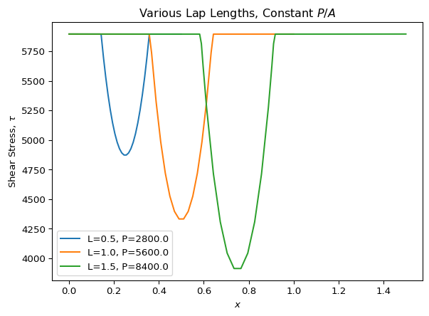
Here, we see that for all three overlap lengths considered, the adhesive at the ends of the lap is plastic and that there’s an elastic “trough” in the middle of each joint. At this point, we might be tempted to declare that all of the joints are able to carry at least the same average shear stress ($P/A$), but before we do so, let’s look at the shear strain in the adhesive layer for each of these cases.

for Li in np.linspace(0.5, 1.5, num=3):
  x_i, gamma_i, tau_i = model(
    t1=t1, t2=t2, ta=ta, L=Li, P=5600*Li
  )
  plt.plot(x_i, gamma_i, label=f"L={Li}, P={5600*Li}")
plt.title("Various Lap Lengths, Constant $P/A$")
plt.ylabel("Shear Strain, $\\gamma$")
plt.xlabel("$x$")
plt.legend()
plt.show()

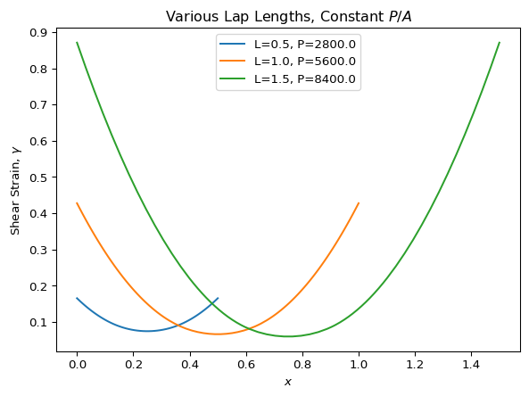
Here we see that the shear strain in the adhesive at the ends of the longest joint is almost 0.9. Think about what that means: the “top” of the adhesive layer has moved sideways relative to the “bottom” of the layer by an amount almost equal to the thickness of the layer. In other words, that a huge amount of strain.

The ultimate shear strain is going to depend on the type of adhesive we’re using, as well as the environmental conditions (temperature, moisture content, etc.). For a lot of adhesives, the ultimate strain is going to be somewhere in the range of $0.2$ to $0.6$. So, in the three examples shown here, the first overlap length ($L=0.5$) can probably carry this value of $P/A$, the second overlap length ($L=1.0$) might be able to carry it, but the third overlap length ($L=1.5$) almost certainly will fail. This is the reason that you can’t use the average shear stress ($P/A$) to size lap joints.

If you want to play around with this model, I’ve created a widget that implements this model.