I’ve made a few violin bows and a couple cello bows. I’m very much a novice bow maker, but I’m learning. As I’m an engineer, I’m naturally trying to apply engineering principles to bow making, which isn’t necessarily easy since violin bows are actually very complex, despite looking quite simple.

The stiffness of a bow affects what the player is able to do with it. If a bow is too stiff, it becomes nearly unplayable; if it’s too soft, they player can’t apply much force to the string before the stick bottoms out and contacts the string (normally the hair of the bow contacts the string). The stiffness affects how much camber the bow maker must add to the stick. The wrong combination of stiffness and camber can lead to a torsional-bending buckling mode, which will make the bow unplayable. The mass and mass distribution of the bow has a large effect on playability. Plus, the aesthetics of the bow are of importance. As I said, a bow is quite complex.

The “standard” wood for making violin bows has been pernambuco for the past 250 years. However, the tree that produces this wood is endangered and hence this wood is difficult to obtain. I’ve been making bows out of other types of wood — mostly ipe and snakewood. In order for a bow made from ipe to have the same stiffness as a bow made from pernambuco, the dimensions need to be altered. Hence, having a good understanding between the taper of the stick and the resulting stiffness is important.

Taper

Henry Saint-George provides a procedure for calculating the taper of a bow based on measurements of Tourte bows ( SaintGeorge (1896) ). In this procedure, the bow is divided into 12 (unequal) segments. Referring to the figure below (reproduced from Saint-George’s book), line AC is constructed perpendicular to the bow with a length of 110 mm. A second line BD is constructed perpendicular to the stick at the other end. Saint-George indicates that the line BD is 22 mm when the total length (AB) is 700 mm. A compass is used to draw the arc Ce. A line perpendicular to the stick is then constructed starting from point e and terminating at the line CD. The compass is re-set to draw the arc fg and the process is repeated. The points A, e, g, i, k, etc. are the points at which the diameter of the bow is set. At points A and e, the diameter are set equal to one another. At points y and B, they are equal to another fixed value. The diameter at the remaining points are each decremented by a fixed value. But, since those points are not uniformly spaced, the taper is not linear, but instead accelerates along the length of the stick.

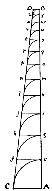
This procedure seems quite complicated. However, the keen reader might recognize that the points along the stick form a geometric series. The keen reader may also recognize that the values 22 mm and 700 mm cannot both be taken as fixed: if you change the length of the bow (which affects the slope of the line CD), you also need to change the length of line BD, otherwise the procedure described above will not produce the correct overall length.

The sum of each of these segments is given by:

$$ L = \sum_{k=0}^{12} C r^k = C\left(\frac{r^{12}-1}{r-1}\right) $$

Here, the value C is selected as 110 mm and the value of $r$ needs to be found based on the value of $L$ chosen. This can be done numerically in Python. The following code does that, then computes the points and the diameters of the bow:

import scipy.optimize

length = 700.
length_constant = 110.
d_butt = 8.6
d_head = 5.6

r = scipy.optimize.root(
    lambda r: length_constant * (r**12 - 1) / (r - 1) - length,
    22
).x[0]
print(f"Found r = {r}\n")

x_points = [0.] * 13
d_points = [0.] * 13

for i in range(13):
    if i == 0:
        d_points[i] = d_butt
    else:
        x_points[i] = length_constant * (r**i - 1) / (r - 1)
        d_points[i] = d_butt + (d_head - d_butt) * (i - 1.) / 10.
    if i == 12:
        d_points[i] = d_head

    print(f"x = {x_points[i]:.1f}, d = {d_points[i]:.2f}")

Found r = 0.8741349707251251

x = 0.0, d = 8.60
x = 110.0, d = 8.60
x = 206.2, d = 8.30
x = 290.2, d = 8.00
x = 363.7, d = 7.70
x = 427.9, d = 7.40
x = 484.0, d = 7.10
x = 533.1, d = 6.80
x = 576.0, d = 6.50
x = 613.5, d = 6.20
x = 646.3, d = 5.90
x = 675.0, d = 5.60
x = 700.0, d = 5.60

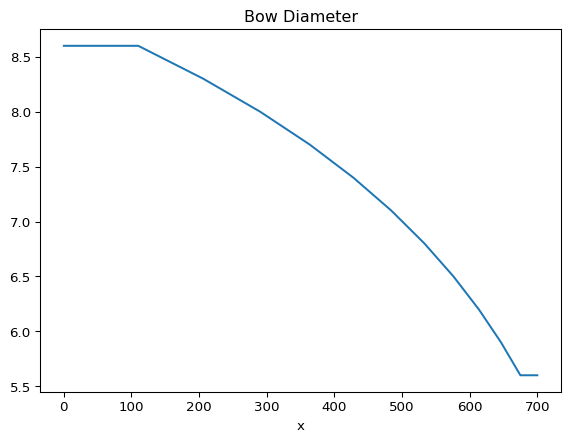
We can plot the diameter of the stick:

import matplotlib.pyplot as plt

plt.plot(x_points, d_points)
plt.title("Bow Diameter")
plt.xlabel("x")
plt.show()

Stiffness

Section Properties

Bows are either (approximately) round or octagonal in cross-section. The area moment of inertia of each of these are as follows ( Oberg et al. (2000) ):

Of course, when determining the stiffness of the bow, the modulus of elasticity also needs to be known. From my research, the modulus of elasticity of pernambuco is about 30 GPa. From my measurements, the modulus of elasticity of ipe is about 20 GPa.

Finite Element Method

In order to determine the stiffness of the stick, we’ll use the finite element method with tapered beam elements. This analysis will be done in two dimensions. We’ll define a node at each of the x points found in the previous calculation of bow taper with a tapered beam element connecting adjacent nodes. The diameter (or width across flats in the case of an octagonal cross-section) is known at each of the nodes. Our model will assume that the variation in the diameter is linear between nodes.

The following derivation is based on Chapter 3 from Cook et al. (2001) , but differs since the elements are tapered beams instead of constant section beams.

Each node will have two degrees of freedom: a transverse displacement and a rotation. The degrees of freedom associated with a single element (which connects two nodes) is thus:

$$ [d] = \left[ \matrix{ \nu_1 & \theta_1 & \nu_2 & \theta_2 } \right] $$

Some of the algebra that we’ll use in the following derivation gets a bit tedious, so we’ll use the symbolic mathematics package sympy to help us:

import sympy

# Due to the way that my blogging platform works, we need to
# define a new function for printing symbolic math:
def sym_print(x):
    print('$${}$$'.format(sympy.printing.latex(x)))

The shape function for our element is a function of the element length $L$ and the position along the element $x$ and is given by:

L = sympy.var("L")
x = sympy.var("x")

B = sympy.Matrix([[
    -6 / L**2 + 12 * x / L**3,
    -4 / L + 6 * x / L**2,
    6 / L**2 - 12 * x / L**3,
    -2 / L + 6 * x / L**2
]])
sym_print(B)

$$\left[\begin{matrix}- \frac{6}{L^{2}} + \frac{12 x}{L^{3}} & - \frac{4}{L} + \frac{6 x}{L^{2}} & \frac{6}{L^{2}} - \frac{12 x}{L^{3}} & - \frac{2}{L} + \frac{6 x}{L^{2}}\end{matrix}\right]$$

For the purpose of stiffness calculations, we’re idealizing the taper of the bow so that within each element the taper is linear. This means that the diameter of the stick at the point $x$ is given by the following. Note that in this section, $x$ and $L$ refer to the distance along the length of the element dn the length of the element, respectively, rather than the dimensions of the bow.

$$ d = d_1 + \frac{x}{L}\left(d_2 - d_1\right) $$

where $d_1$ and $d_2$ are the diameters at nodes 1 and 2, respectively. So that we don’t have to carry around so many variables, we’ll define the variable $\beta$ such that:

$$ d = d_1 + \beta x $$

As we found earlier, for both circular sections and octagonal sections, the moment of inertia ($I$) is a function of $d^4$. We’ll define a new variable $\alpha$ such that:

$$ EI = \alpha d^4 $$

Combining the previous two equations and entering this into sympy, we get:

alpha = sympy.var("\\alpha")
d1 = sympy.var("d_1")
beta = sympy.var("\\beta")
EI = alpha * (d1 + beta * x)**4
sym_print(EI)

$$\alpha \left(\beta x + d_{1}\right)^{4}$$

The stiffness matrix for the element is given by:

$$ [k] = \int_0^L \left[B\right]^T EI \left[B\right] dx $$

Solving and simplifying this using sympy, we get the following. The stiffness matrix is a 4x4 matrix that is quite complex, so we’ll show one column at a time in this post:

k = sympy.simplify(
    sympy.integrate(B.T * EI * B, (x, 0, L))
)

# The first column
sym_print(k[:,0])

$$\left[\begin{matrix}\frac{12 \alpha \left(11 L^{4} \beta^{4} + 49 L^{3} \beta^{3} d_{1} + 84 L^{2} \beta^{2} d_{1}^{2} + 70 L \beta d_{1}^{3} + 35 d_{1}^{4}\right)}{35 L^{3}}\frac{2 \alpha \left(19 L^{4} \beta^{4} + 84 L^{3} \beta^{3} d_{1} + 147 L^{2} \beta^{2} d_{1}^{2} + 140 L \beta d_{1}^{3} + 105 d_{1}^{4}\right)}{35 L^{2}}\frac{12 \alpha \left(- 11 L^{4} \beta^{4} - 49 L^{3} \beta^{3} d_{1} - 84 L^{2} \beta^{2} d_{1}^{2} - 70 L \beta d_{1}^{3} - 35 d_{1}^{4}\right)}{35 L^{3}}\frac{2 \alpha \left(47 L^{4} \beta^{4} + 210 L^{3} \beta^{3} d_{1} + 357 L^{2} \beta^{2} d_{1}^{2} + 280 L \beta d_{1}^{3} + 105 d_{1}^{4}\right)}{35 L^{2}}\end{matrix}\right]$$

# The second column
sym_print(k[:,1])

$$\left[\begin{matrix}\frac{2 \alpha \left(19 L^{4} \beta^{4} + 84 L^{3} \beta^{3} d_{1} + 147 L^{2} \beta^{2} d_{1}^{2} + 140 L \beta d_{1}^{3} + 105 d_{1}^{4}\right)}{35 L^{2}}\frac{4 \alpha \left(3 L^{4} \beta^{4} + 14 L^{3} \beta^{3} d_{1} + 28 L^{2} \beta^{2} d_{1}^{2} + 35 L \beta d_{1}^{3} + 35 d_{1}^{4}\right)}{35 L}\frac{2 \alpha \left(- 19 L^{4} \beta^{4} - 84 L^{3} \beta^{3} d_{1} - 147 L^{2} \beta^{2} d_{1}^{2} - 140 L \beta d_{1}^{3} - 105 d_{1}^{4}\right)}{35 L^{2}}\frac{2 \alpha \left(13 L^{4} \beta^{4} + 56 L^{3} \beta^{3} d_{1} + 91 L^{2} \beta^{2} d_{1}^{2} + 70 L \beta d_{1}^{3} + 35 d_{1}^{4}\right)}{35 L}\end{matrix}\right]$$

# The third column
sym_print(k[:,2])

$$\left[\begin{matrix}\frac{12 \alpha \left(- 11 L^{4} \beta^{4} - 49 L^{3} \beta^{3} d_{1} - 84 L^{2} \beta^{2} d_{1}^{2} - 70 L \beta d_{1}^{3} - 35 d_{1}^{4}\right)}{35 L^{3}}\frac{2 \alpha \left(- 19 L^{4} \beta^{4} - 84 L^{3} \beta^{3} d_{1} - 147 L^{2} \beta^{2} d_{1}^{2} - 140 L \beta d_{1}^{3} - 105 d_{1}^{4}\right)}{35 L^{2}}\frac{12 \alpha \left(11 L^{4} \beta^{4} + 49 L^{3} \beta^{3} d_{1} + 84 L^{2} \beta^{2} d_{1}^{2} + 70 L \beta d_{1}^{3} + 35 d_{1}^{4}\right)}{35 L^{3}}\frac{2 \alpha \left(- 47 L^{4} \beta^{4} - 210 L^{3} \beta^{3} d_{1} - 357 L^{2} \beta^{2} d_{1}^{2} - 280 L \beta d_{1}^{3} - 105 d_{1}^{4}\right)}{35 L^{2}}\end{matrix}\right]$$

# The fourth column
sym_print(k[:,3])

$$\left[\begin{matrix}\frac{2 \alpha \left(47 L^{4} \beta^{4} + 210 L^{3} \beta^{3} d_{1} + 357 L^{2} \beta^{2} d_{1}^{2} + 280 L \beta d_{1}^{3} + 105 d_{1}^{4}\right)}{35 L^{2}}\frac{2 \alpha \left(13 L^{4} \beta^{4} + 56 L^{3} \beta^{3} d_{1} + 91 L^{2} \beta^{2} d_{1}^{2} + 70 L \beta d_{1}^{3} + 35 d_{1}^{4}\right)}{35 L}\frac{2 \alpha \left(- 47 L^{4} \beta^{4} - 210 L^{3} \beta^{3} d_{1} - 357 L^{2} \beta^{2} d_{1}^{2} - 280 L \beta d_{1}^{3} - 105 d_{1}^{4}\right)}{35 L^{2}}\frac{4 \alpha \left(17 L^{4} \beta^{4} + 77 L^{3} \beta^{3} d_{1} + 133 L^{2} \beta^{2} d_{1}^{2} + 105 L \beta d_{1}^{3} + 35 d_{1}^{4}\right)}{35 L}\end{matrix}\right]$$

We can now write a function that outputs the stiffness matrix for a tapered beam element:

import numpy as np

def elm_k(L, d1, d2, alpha):
    b = (d2 - d1) / L
    return 2 * alpha / (35*L**3) * np.array(
        [
            [
                6*(11*L**4*b**4 + 49*L**3*b**3*d1 + 84*L**2*b**2*d1**2 + 70*L*b*d1**3 + 35*d1**4),
                L*(19*L**4*b**4 + 84*L**3*b**3*d1 + 147*L**2*b**2*d1**2 + 140*L*b*d1**3 + 105*d1**4),
                6*(-11*L**4*b**4 - 49*L**3*b**3*d1 - 84*L**2*b**2*d1**2 - 70*L*b*d1**3 - 35*d1**4),
                L*(47*L**4*b**4 + 210*L**3*b**3*d1 + 357*L**2*b**2*d1**2 + 280*L*b*d1**3 + 105*d1**4)
            ],
            [
                L*(19*L**4*b**4 + 84*L**3*b**3*d1 + 147*L**2*b**2*d1**2 + 140*L*b*d1**3 + 105*d1**4),
                2*L**2*(3*L**4*b**4 + 14*L**3*b**3*d1 + 28*L**2*b**2*d1**2 + 35*L*b*d1**3 + 35*d1**4),
                L*(-19*L**4*b**4 - 84*L**3*b**3*d1 - 147*L**2*b**2*d1**2 - 140*L*b*d1**3 - 105*d1**4), 
                L**2*(13*L**4*b**4 + 56*L**3*b**3*d1 + 91*L**2*b**2*d1**2 + 70*L*b*d1**3 + 35*d1**4)
            ],
            [
                6*(-11*L**4*b**4 - 49*L**3*b**3*d1 - 84*L**2*b**2*d1**2 - 70*L*b*d1**3 - 35*d1**4),
                L*(-19*L**4*b**4 - 84*L**3*b**3*d1 - 147*L**2*b**2*d1**2 - 140*L*b*d1**3 - 105*d1**4),
                6*(11*L**4*b**4 + 49*L**3*b**3*d1 + 84*L**2*b**2*d1**2 + 70*L*b*d1**3 + 35*d1**4),
                L*(-47*L**4*b**4 - 210*L**3*b**3*d1 - 357*L**2*b**2*d1**2 - 280*L*b*d1**3 - 105*d1**4)
            ],
            [
                L*(47*L**4*b**4 + 210*L**3*b**3*d1 + 357*L**2*b**2*d1**2 + 280*L*b*d1**3 + 105*d1**4),
                L**2*(13*L**4*b**4 + 56*L**3*b**3*d1 + 91*L**2*b**2*d1**2 + 70*L*b*d1**3 + 35*d1**4),
                L*(-47*L**4*b**4 - 210*L**3*b**3*d1 - 357*L**2*b**2*d1**2 - 280*L*b*d1**3 - 105*d1**4),
                2*L**2*(17*L**4*b**4 + 77*L**3*b**3*d1 + 133*L**2*b**2*d1**2 + 105*L*b*d1**3 + 35*d1**4)
            ]
        ]
    )

Stroup Test

The Stroup Test is a way of testing the stiffness of the stick of a bow. In this test, the bow is mounted in a jig that supports the stick on two rollers that are 575 mm apart. A transverse force of 2 lb is applied mid-way between the two rollers and the deflection at the force application point is measured. From what I can tell, there were a small number of people advocating this test some time ago, but it has since become quite uncommon — most makers will assess the stiffness of a stick by feel. However, the Stroup Test can be easily implemented using the finite element method for the purpose of assessing relative stiffness of sticks made from different materials with different dimensions.

Implementing the Stroup Test

We already have a list of nodal locations. We’ll choose one of these nodes as the location of one of the supports (we’ll use the second last node for this). We’ll need to ensure that there are two other nodes for the load application point and the other support in the correct location. We’ll likely need to create these nodes and sub-divide the existing elements. We can do this in Python as follows:

x_nodes = []
d_nodes = []

x_s2 = x_points[11]
x_s1 = x_s2 - 575
x_l = x_s2 - 575 / 2

nid_s1 = -1  # storage for node ID of support #1
nid_s2 = -1  # storage for node ID of support #2
nid_l = -1   # storage for node ID of load application

tol = lambda xa, xb: abs(xa - xb) < 1e-3
inside = lambda x, xa, xb: (x - xa) * (x - xb) < 0

for x1, x2, d1, d2 in zip(
    x_points, x_points[1:], d_points, d_points[1:]):
    x_nodes.append(x1)
    d_nodes.append(d1)

    if tol(x_s1, x1):
        nid_s1 = len(x_nodes) - 1
    elif inside(x_s1, x1, x2):
        x_nodes.append(x_s1)
        d_nodes.append(d1 + (x_s1 - x1) / (x2 - x1) * (d2 - d1))
        nid_s1 = len(x_nodes) - 1

    if tol(x_s2, x1):
        nid_s2 = len(x_nodes) - 1
    elif inside(x_s2, x1, x2):
        x_nodes.append(x_s2)
        d_nodes.append(d1 + (x_s2 - x1) / (x2 - x1) * (d2 - d1))
        nid_s2 = len(x_nodes) - 1

    if tol(x_l, x1):
        nid_l = len(x_nodes) - 1
    elif inside(x_l, x1, x2):
        x_nodes.append(x_l)
        d_nodes.append(d1 + (x_l - x1) / (x2 - x1) * (d2 - d1))
        nid_l = len(x_nodes) - 1

x_nodes.append(x_points[-1])
d_nodes.append(d_points[-1])

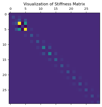
We can now build a stiffness matrix for the model. There are now 15 nodes and each node has 2 DOF, so the matrix will be 30 x 30. We’ll use a sparse matrix. We’ll assume that all elements are round and the material has a modulus of 30 GPa.

k_model= np.zeros((2 * len(x_nodes), 2 * len(x_nodes)))

for i, (x1, x2, d1, d2) in enumerate(
    zip(x_nodes, x_nodes[1:], d_nodes, d_nodes[1:])):
    # Each element connects the two adjacent nodes
    k_elm = elm_k(
        L = x2 - x1,
        d1 = d1,
        d2 = d2,
        alpha = 0.0490874 * 30e3
    )
    for ii in range(4):
        for jj in range(4):
            k_model[i * 2 + ii, i * 2 + jj] += k_elm[ii,jj]

We can visualize the stiffness matrix. As expected, all of the elements are near the diagonal.

plt.matshow(k_model)
plt.title("Visualization of Stiffness Matrix")

Text(0.5, 1.0, 'Visualization of Stiffness Matrix')

Next, we will create the load vector. This vector will have all elements set to zero except for the entry corresponding to the first DOF of the loading node.

p_model = np.zeros(2 * len(x_nodes))
p_model[nid_l * 2] = -8.9075  # 2 lb in N

Next, we’ll take away the constrained DOFs from the stiffness matrix and the load vector. In our case, those DOFs are the transverse displacement of the constrained nodes.

mask = [i for i, _ in enumerate(p_model)
        if i != nid_s1 * 2 and i != nid_s2 * 2]

p_const = p_model[mask]
k_const = k_model[mask, :]
k_const = k_const[:, mask]

Now, we can solve for the deflections:

import scipy.linalg
d_const = scipy.linalg.solve(k_const, p_const)

Now, we can add back in the constrained DOFs into the displacement solution. These will be zero because these DOFs were constrained.

d_model = np.zeros(2 * len(x_nodes))
d_model[mask] = d_const

Now, we can plot the results:

plt.plot(x_nodes, d_model[0::2])
plt.grid()
plt.title("Deflection")
plt.xlabel("x")
plt.ylabel("Vertical Deflection")
plt.show()

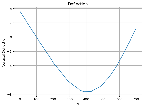
Stroup values are normally given in thousandths of an inch, which we can calculate as follows:

-d_model[nid_l * 2] / 25.4 * 1000

301.20020904559294

Conclusion

This blog post describes a way of numerically finding the relationship between the stiffness of a violin bow and its taper. We used the finite element method to do so. I’m planning on developing an online calculator for performing this computation. I plan to use an early version of py-script to do so, but since I’ve never used py-script, it’s possible that it will take a while to figure it out.