Recently, I wrote a blog post about computing section properties. I discussed using Green’s Theorem to compute the area integrals needed to compute section properties (area, centroid and moment of inertia) and I made the guess that this is how commercial software probably computes the section properties of arbitrary shapes. In that previous post, I only considered section bounded by line segments. In this post, I’ll extend that approach to include circular arcs. I’ll also write some Python code for computing the section properties of an arbitrary shape bounded by line and arc segments.
Arcs
For our purposes, we’ll describe an arc using its center point, radius, starting angle and ending angle. The arc will be parameterized using \(\theta\), which will vary between \(\theta_a\) and \(\theta_b\).
We’ll need the derivatives of these functions too:
Area for an Arc
As discsused in the previous blog post, the area can be comuted using Green’s Theorem. The increment of the area attributable to the arc segment is given by:
Centroid of an Arc
Following from the previous blog post, the increment centroid can be computed as follows. Note that the area (\(A\)) here is the area of the entire shape, not the increment in area due to the present segment.
First, in the X axis:
Next, in the Y axis:
Moment of Inertia of an Arc
Following from the previous blog post, the increment moment can be computed as follows. As before, when computing the moment of inertia, the coordinates need to be shifted to coincide with the centroid. There is a closed-form solution, however it is quite complicated, so we’ll use quadrature instead. The integrals are as follows:
Implementation in Python
Now, we’ll implement this in Python so that the section properties of an arbitrary shape bounded by line and arc segments can be computed. We’ll need the following import’s:
import numpy as np
import matplotlib.pyplot as plt
import matplotlib.lines
import matplotlib.patches
import scipy.integrate
from dataclasses import dataclass
from typing import Callable, List, Tuple
Later, we’ll write a class for the shape that will contain
a list of segments that can be either line segments or
arc segments. Both types of segment will inherit from the
same base class (Segment) that will have the following
two methods:
class Segment:
    def draw(self, ax):
        raise NotImplementedError

    def calc_delta_area(self):
        raise NotImplementedError

    def calc_delta_centroid_x_2a(self):
        raise NotImplementedError

    def calc_delta_centroid_y_2a(self):
        raise NotImplementedError

    def calc_delta_i_yy(self, centroid):
        raise NotImplementedError

    def calc_delta_i_xx(self, centroid):
        raise NotImplementedError
First, let’s implement a line segment, as that is fairly straight forward. This is from the previous post.
@dataclass
class Line(Segment):
    a: Tuple[float, float]
    b: Tuple[float, float]

    def draw(self, ax):
        line = matplotlib.lines.Line2D(
            (self.a[0], self.b[0]), (self.a[1], self.b[1])
        )
        ax.add_line(line)

    def calc_delta_area(self):
        xa, ya = self.a
        xb, yb = self.b
        return 1 / 2 * (xa * (yb - ya) - ya * (xb - xa))

    def calc_delta_centroid_x_2a(self):
        xa, ya = self.a
        xb, yb = self.b
        return (xa**2 + xa * (xb - xa) + 1 / 3 * (xb - xa)**2) * (yb - ya)

    def calc_delta_centroid_y_2a(self):
        xa, ya = self.a
        xb, yb = self.b
        return -(ya**2 + ya * (yb - ya) + 1 / 3 * (yb - ya)**2) * (xb - xa)

    def calc_delta_i_yy(self, centroid):
        xa, ya = np.array(self.a) - np.array(centroid)
        xb, yb = np.array(self.b) - np.array(centroid)
        return 1 / 3 * (xa**3 + 3 / 2 * xa**2 * (xb - xa) + xa * (xb - xa)**2 + 1 / 4 * (xb - xa)**3) * (yb - ya)

    def calc_delta_i_xx(self, centroid):
        xa, ya = np.array(self.a) - np.array(centroid)
        xb, yb = np.array(self.b) - np.array(centroid)
        return -1 / 3 * (ya**3 + 3 / 2 * ya**2 * (yb - ya) + ya * (yb - ya)**2 + 1 / 4 * (yb - ya)**3) * (xb - xa)
While the basic math for the arc segment is given above, it requires some thought. The endpoints of the arc are given in terms of two angles, but it’s important to pay attention to whether the path of the arc is in the clockwise or counterclockwise direction, and it’s important to note that there are \(2^\circ\) between \(179^\circ\) and \(-179^\circ\), not \(358^\circ\).
To address this, in addition to the endpoints, we’ll include a
boolean variable indicating the direction (ccw = True) and
apply the following rules. Note that we’ll be using the function
np.atan2 to returns angles in the range \(\left[-\pi, \pi\right]\) radians,
so we’ll assume that all angles are in that range.
- Direction: conterclockwise
- \(\theta_a < \theta_b\): process as-is
- \(\theta_a > \theta_b\): wraps around \(\pi\); break into two arcs with \(\theta\) ranges \(\left(\theta_a, \pi\right)\) and \(\left(-\pi, \theta_b\right)\).
- Direction: clockwise
- \(\theta_a < \theta_b\): wraps around \(\pi\); break into two arcs with \(\theta\) ranges \(\left(\theta_a, -\pi\right)\) and \(\left(\pi, \theta_b\right)\).
- \(\theta_a > \theta_b\): process as-is
@dataclass
class Arc(Segment):
    center: Tuple[float, float]
    r: float
    theta_a: float
    theta_b: float
    ccw: bool

    def draw(self, ax):
        theta_a=self.theta_a if self.ccw else self.theta_b
        theta_b=self.theta_b if self.ccw else self.theta_a
        patch = matplotlib.patches.Arc(
            self.center,
            2. * self.r,
            2. * self.r,
            theta1=theta_a * 180. / np.pi,
            theta2=theta_b * 180. / np.pi)
        ax.add_patch(patch)

    def _call_on_normalized_range(self, fcn: Callable) -> float:
        # fcn should accept the arguments theta_a, theta_b
        if self.ccw:
            if self.theta_a < self.theta_b:
                return float(fcn(self.theta_a, self.theta_b))
            else:
                return float(fcn(self.theta_a, np.pi) + fcn(-np.pi, self.theta_b))
        else:
            if self.theta_a < self.theta_b:
                return float(fcn(self.theta_a, -np.pi) + fcn(np.pi, self.theta_b))
            else:
                return float(fcn(self.theta_a, self.theta_b))

    def calc_delta_area(self):
        def _calc_delta_area(theta_a: float, theta_b: float):
            return float(self.center[0] * self.r / 2 * (np.sin(theta_b) - np.sin(theta_a)) \
                - self.center[1] * self.r / 2 * (np.cos(theta_b) - np.cos(theta_a)) \
                + self.r**2 / 2 * (theta_b - theta_a))
        return self._call_on_normalized_range(_calc_delta_area)

    def calc_delta_centroid_x_2a(self):
        def _calc_delta_centroid_x_2a(theta_a: float, theta_b: float):
            return self.r * (
                (self.center[0]**2 + self.r**2) * (np.sin(theta_b) - np.sin(theta_a))
                + self.center[0] * self.r * (
                    theta_b - theta_a +
                    1. / 2. * np.sin(2. * theta_b) - 1. / 2. * np.sin(2. * theta_a)
                )
                - self.r**2 / 3. * (np.sin(theta_b)**3 - np.sin(theta_a)**3)
            )
        return self._call_on_normalized_range(_calc_delta_centroid_x_2a)

    def calc_delta_centroid_y_2a(self):
        def _calc_delta_centroid_y_2a(theta_a: float, theta_b: float):
            return self.r * (
                -(self.center[1]**2 + self.r**2) * (np.cos(theta_b) - np.cos(theta_a))
                + self.center[1] * self.r * (
                    theta_b - theta_a
                    - 1. / 2. * np.sin(2. * theta_b) + 1. / 2. * np.sin(2. * theta_a)
                )
                + self.r**2 / 3. * (np.cos(theta_b)**3 - np.cos(theta_a)**3)
            )
        return self._call_on_normalized_range(_calc_delta_centroid_y_2a)

    def calc_delta_i_yy(self, centroid):
        xc = self.center[0] - centroid[0]

        def integral(a, b):
            return scipy.integrate.quad(
                lambda theta: self.r / 3. * (xc + self.r * np.cos(theta))**3 * np.cos(theta),
                a, b)[0]

        return self._call_on_normalized_range(integral)

    def calc_delta_i_xx(self, centroid):
        yc = self.center[1] - centroid[1]

        def integral(a, b):
            return scipy.integrate.quad(
                lambda theta: self.r / 3. * (yc + self.r * np.sin(theta))**3 * np.sin(theta),
                a, b)[0]

        return self._call_on_normalized_range(integral)
Next, we’ll create the class Shape that serves as a collection
of objects of type Segment and will allow the user to compute the
section properties.
This class will also contain methods to plot and summarize the section.
class Shape:
    segments: List[Segment]
    start: np.array
    current: np.array

    def __init__(self, start: Tuple[float, float]):
        self.segments = []
        self.start = np.array(start)
        self.current = np.array(start)

    def line_to(self, end: Tuple[float, float]):
        pass

    def arc_center_end(self, center: Tuple[float, float], end: Tuple[float, float], ccw: bool):
        center = np.array(center)
        end = np.array(end)
        r = float(np.linalg.norm(center - self.current))
        theta1 = np.atan2(
            (self.current - center)[1],
            (self.current - center)[0]
        )
        theta2 = np.atan2(
            (end - center)[1],
            (end - center)[0]
        )
        self.segments.append(
            Arc(center, r, theta1, theta2, ccw)
        )
        self.current = center + r * np.array([np.cos(theta2), np.sin(theta2)])

    def line_to(self, end: Tuple[float, float]):
        self.segments.append(
            Line(self.current, end)
        )
        self.current = np.array(end)

    def close(self):
        self.line_to(self.start)

    def plot(self):
        fig, ax = plt.subplots()
        for s in self.segments:
            s.draw(ax)
        ax.autoscale(axis="both")
        ax.set_aspect("equal")

    def compute_area(self):
        if not np.array_equal(self.current, self.start):
            raise RuntimeError("Shape is not closed")
        return float(sum([s.calc_delta_area() for s in self.segments]))

    def compute_centroid(self):
        if not np.array_equal(self.current, self.start):
            raise RuntimeError("Shape is not closed")
        area = self.compute_area()
        return (float(sum([s.calc_delta_centroid_x_2a() for s in self.segments])) / (2 * area),
            float(sum([s.calc_delta_centroid_y_2a() for s in self.segments])) / (2 * area))

    def compute_moment_of_inertia(self):
        if not np.array_equal(self.current, self.start):
            raise RuntimeError("Shape is not closed")
        centroid = self.compute_centroid()
        return (float(sum([s.calc_delta_i_xx(centroid) for s in self.segments])),
            float(sum([s.calc_delta_i_yy(centroid) for s in self.segments])))

    def summarize(self):
        centroid = self.compute_centroid()
        inertia = self.compute_moment_of_inertia()
        return "Area = {:.4f}\nCentroid = ({:.4f}, {:.4f})\nI = ({:.4f}, {:.4f})".format(
            self.compute_area(),
            centroid[0], centroid[1],
            inertia[0], inertia[1]
        )
Examples
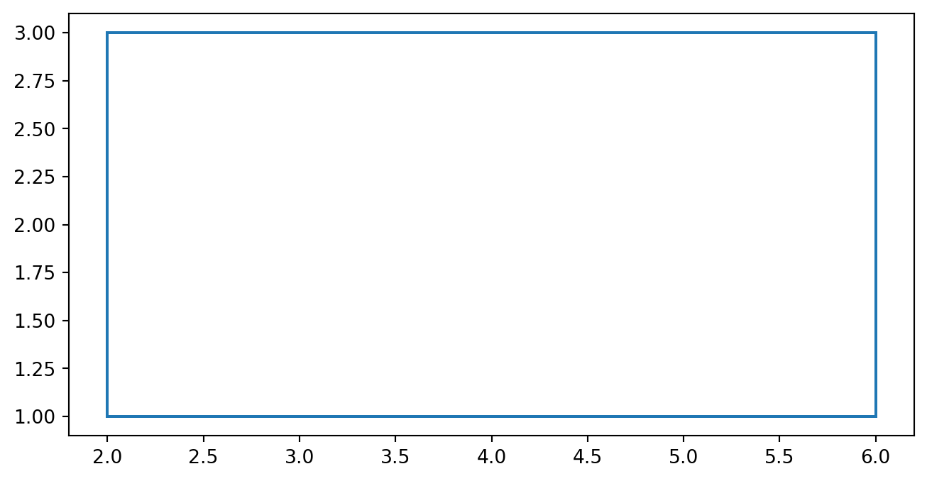
To check the implementation above, let’s try a few examples. First, a simple rectangle.
rect_cw = Shape((2, 3))
rect_cw.line_to((6, 3))
rect_cw.line_to((6, 1))
rect_cw.line_to((2, 1))
rect_cw.close()
rect_cw.plot()
print(rect_cw.summarize())
Area = -8.0000
Centroid = (4.0000, 2.0000)
I = (-2.6667, -10.6667)

The magnitude of the area and moments of inertia are correct, however they’re negative. That’s weird: how can an area be negative? This is caused by the fact that the points defined above are sorted in the clockwise direction. The points are top-left, top-right, lower-right followed by lower left — that’s clockwise. To rectify this, we’ll just reverse the points so that they are ordered in the counterclockwise direction:
rect_ccw = Shape((2, 1))
rect_ccw.line_to((6, 1))
rect_ccw.line_to((6, 3))
rect_ccw.line_to((2, 3))
rect_ccw.close()
rect_ccw.plot()
print(rect_ccw.summarize())
Area = 8.0000
Centroid = (4.0000, 2.0000)
I = (2.6667, 10.6667)
That’s the result that we expect.
Next, let’s try a shape that contains an arc. We’ll start with a semi-circle.
semicirc = Shape((6, 3))
semicirc.arc_center_end((4, 3), (2, 3), True)
semicirc.close()
semicirc.plot()
print(semicirc.summarize())
Area = 6.2832
Centroid = (4.0000, 3.8488)
I = (1.7561, 6.2832)
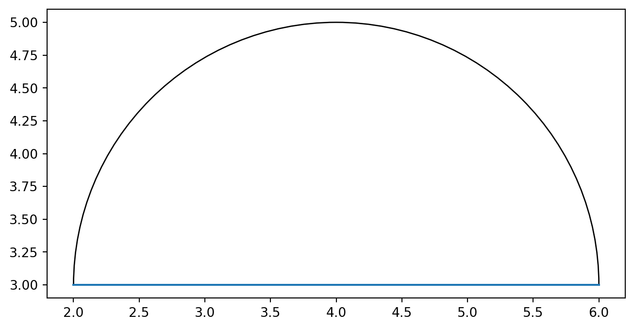
The section properties of a semicircle should be
| Property | Formula | Result |
|---|---|---|
| Area | \(\frac{\pi r^2}{2}\) | 6.283 |
| \(\bar{X}\) | \(x_c\) | 4.000 |
| \(\bar{Y}\) | \(\frac{4}{3\pi} R + y_c\) | 3.849 |
| \(I_{XX}\) | \(0.1098 r^4\) | 1.757 |
| \(I_{YY}\) | \(\frac{\pi}{8} r^4\) | 6.283 |
That was all correct.
Next, let’s try a shape that includes both line segments and an arc. We’ll simply stack the rectagle and arc above on top of each other.
stacked_shape = Shape((2, 1))
stacked_shape.line_to((6, 1))
stacked_shape.line_to((6, 3))
stacked_shape.arc_center_end((4, 3), (2, 3), True)
stacked_shape.close()
stacked_shape.plot()
print(stacked_shape.summarize())
Area = 14.2832
Centroid = (4.0000, 2.8133)
I = (16.4520, 16.9499)
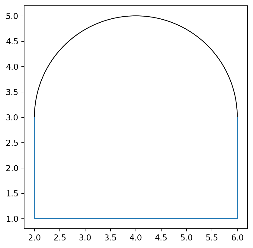
The expected section properties can be computed based on the previous results:
| Element | Area | \(\bar{Y_i}\) | \(A \bar{Y_i}\) | \(I_i\) | \(A_i\left(Y_i - \bar{Y}\right)^2\) |
|---|---|---|---|---|---|
| Rectangle | 8.000 | 2.000 | 16.000 | 2.667 | 5.288 |
| Semicircle | 6.283 | 3.849 | 24.183 | 1.756 | 6.744 |
| \(\sum\) | 14.283 | 40.183 | 4.423 | 12.032 |
The total moment of inertia is:
This matches the value computed by the Python code above.
The code in this blog post is certainly not production-ready since it performs very limited input validation and other error checking. However, it does demonstrate this technique of computing section properties. This approach could be extended even further by allowing for shapes bounded by other segments, such as eliptical arcs, cubic splines or any number of other contours.