Earlier, I wrote a post about using a likelihood-based approach to calculating Basis values. In that post, I hinted that likelihood-based approaches can be useful when dealing with censored data.
First of all, what does censoring mean? It means that the value reported is either artificially high or artificially low. There are a few reasons that this could happen. It happens often with lifetime data: with fatigue tests, you set a number of cycles at which the specimen “runs out” and you stop the test; with studies of mortality, some of the subjects will still be alive when you do the analysis. In these cases, the true value is greater than the observed result, but you don’t know by how much. These are examples of right-censored data.
Data can also be left-censored, meaning that the true value is less than the observed value. This can happen if some of the values are too small to be measured. Perhaps the instrument that you’re using can’t detect values below a certain amount.
There is also interval-censored data. This often occurs in survey data. For example, you might have data for individuals aged 40-44, but you don’t know where they fall within that range.
In this post, we’re going to deal with right-censored data.
At my day job, I often deal with data from testing of metallic inserts installed in honeycomb sandwich panel. These metallic inserts have a hole in their centers that will accept a screw. Their purpose is to allow a screw to be fastened to the panel, and the strength of this connections is one of the important considerations.
We determine the strength of the insert through testing. The usual test coupon that we use has two of these inserts installed, and we pull them away from each other to measure the shear strength. This is a convenient way of applying the load, but I’ve long thought that it must give low results. The loading of the coupon looks like this:
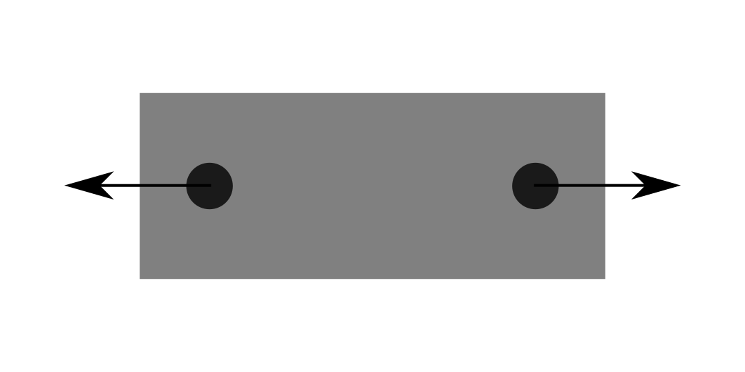
The reason that I’ve thought that this test method will give artificially low results is the fact that there are two inserts. The test ends when either one of these two insert fails: the other insert must be stronger than the one that failed first.
To illustrate this, let’s do a slightly silly thought experiment. Let’s imagine that we’re making a set of these coupons. We decide that we’re going to install one insert in each coupon first, then come back tomorrow and install the other insert in each coupon. Tomorrow comes around, and we decide to let the brand new intern install the second insert. The intern hasn’t yet been fully trained, and they accidentally install the wrong type of insert in teh second hole, but unfortunately they look identical to the correct type. The correct type of insert has a strength that is always \(1000 lbf\), but we don’t know that yet. The wrong type of insert always has a strength of exactly \(500 lbf\). When we do our tests, all of the coupons fail on the side that the intern installed (the wrong insert) and the strength of each coupon is \(500 lbf\). We conclude that the mean strength of these inserts is \(500 lbf\) with a very low variance.
But, we’d be wrong.
In this thought experiment, the actual mean strength of the inserts (considering both the correct and incorrect types of inserts) is \(750 lbf\) and there’s actually a pretty high variance. We were simply unable to observe the strength of the stronger screws because of censoring.
In a more realistic case, we’re actually going to be dealing with parts that have strengths drawn from the same continuous distribution. As we move on, we’re going to assume that the strength of each individual insert is a random variable drawn from the same continuous distribution (that is, they are IID).
Let’s create some simulated data. We’ll start by loading a few R packages that we’ll need.
library(tidyverse)
library(cmstatr)
library(stats4)
Next, we’ll create a sample of \(40\) simulated insert strengths. These will be drawn from a normal distribution with a mean of \(1000\) and a standard deviation of \(100\).
pop_mean <- 1000
pop_sd <- 100

set.seed(123)  # make this example reproducible

strength <- rnorm(40, pop_mean, pop_sd)
Now let’s calculate the mean of this sample. We expect it to be fairly close to 1000, and indeed it is.
mean(strength)
## [1] 1004.518
And we can also calculate the standard deviation:
sd(strength)
## [1] 89.77847
For the strength of most aircraft structures, we are concerned with a lower tolerance bound of the strength. For multiple load-path structure, we need to calculate the B-Basis strength, which is the \(95/%\) lower confidence bound on the 10-th percentile of the strength.
Since we know the actual strength of all 40 inserts, we can calculate the B-Basis based on these actual insert strengths. Ideally, the B-Basis value that we calculate later will be close to this value.
basis_normal(x = strength)
## `outliers_within_batch` not run because parameter `batch` not specified
## `between_batch_variability` not run because parameter `batch` not specified

##
## Call:
## basis_normal(x = strength)
##
## Distribution:  Normal    ( n = 40 )
## B-Basis:   ( p = 0.9 , conf = 0.95 )
## 852.1482
Now, we’ll take these \(40\) insert strengths and put them into \(20\) coupons: each with two inserts. The observed coupon strength will be set to the lower of the two inserts installed in that coupon, because the coupon will fail as soon as either one of the installed inserts fails.
dat <- data.frame(
  ID = 1:20,
  strength1 = strength[1:20],
  strength2 = strength[21:40]
) %>%
  rowwise() %>%
  mutate(strength_observed = min(strength1, strength2)) %>%
  ungroup()
dat
## # A tibble: 20 × 4
##       ID strength1 strength2 strength_observed
##    <int>     <dbl>     <dbl>             <dbl>
##  1     1      944.      893.              893.
##  2     2      977.      978.              977.
##  3     3     1156.      897.              897.
##  4     4     1007.      927.              927.
##  5     5     1013.      937.              937.
##  6     6     1172.      831.              831.
##  7     7     1046.     1084.             1046.
##  8     8      873.     1015.              873.
##  9     9      931.      886.              886.
## 10    10      955.     1125.              955.
## 11    11     1122.     1043.             1043.
## 12    12     1036.      970.              970.
## 13    13     1040.     1090.             1040.
## 14    14     1011.     1088.             1011.
## 15    15      944.     1082.              944.
## 16    16     1179.     1069.             1069.
## 17    17     1050.     1055.             1050.
## 18    18      803.      994.              803.
## 19    19     1070.      969.              969.
## 20    20      953.      962.              953.
Let’s look at the summary statistics for this data:
dat %>%
  summarise(
    mean = mean(strength_observed),
    sd = sd(strength_observed),
    cv = cv(strength_observed)
  )
## # A tibble: 1 × 3
##    mean    sd     cv
##   <dbl> <dbl>  <dbl>
## 1  954.  75.1 0.0788
Hmmm. We see the mean is much lower than the mean of the individual insert strength. Remember that the mean insert strength was \(1005\), but the mean strength of the coupons is \(954\).
Next, we’ll naively calculate a B-Basis value from the measured strength. We’ll assume a normal distribution.
dat %>%
  basis_normal(strength_observed)
##
## Call:
## basis_normal(data = ., x = strength_observed)
##
## Distribution:  Normal    ( n = 20 )
## B-Basis:   ( p = 0.9 , conf = 0.95 )
## 809.1911
We’ll just keep this number in mind for now and we’ll move on to the idea of using a likelihood-based approach to calculate a B-Basis value, considering the fact that this data is censored.
The way that this data is censored might not be immediately obvious. But, each time we test one of these coupons, which contain two inserts, we actually get two pieces of data. We get the strength of one of the inserts. This is an exact value. But we also get a second piece of data. We know that the strength of the other insert is at least as high as the one that failed first. This is a right censored value.
In the previous post, I gave an expression for the likelihood function. However, that function only considers exact observations. The expression for the likelihood, considering censored data as follows (see Meeker et al. (2017) ).
Where \(f()\) is the probability density function and \(F()\) is the cumulative density function.
We can implement a log-likelihood function based on this in R as follows:
log_likelihood_normal <- function(mu, sig, x, censored) {
  suppressWarnings(
    sum(map2_dbl(x, censored, function(xi, ci) {
      if (ci == "exact") {
        dnorm(xi, mean = mu, sd = sig, log = TRUE)
      } else if (ci == "left") {
        pnorm(xi, mean = mu, sd = sig, log.p = TRUE)
      } else if (ci == "right") {
        pnorm(xi, mean = mu, sd = sig, log.p = TRUE,
               lower.tail = FALSE)
      } else {
        stop("Invalid value of `censored`")
      }
    }))
  )
}
We can use this log-likelihood function to find the maximum-likelihood
estimates (MLE) of the population parameters using the stats4::mle()
function. First, we’ll find the MLE based only on the observed strength
of each coupon, taken as a single exact value.
mle(
  function(mu, sig) {
    -log_likelihood_normal(mu, sig, dat$strength_observed, "exact")
  },
  start = c(1000, 100)
)
##
## Call:
## mle(minuslogl = function(mu, sig) {
##     -log_likelihood_normal(mu, sig, dat$strength_observed, "exact")
## }, start = c(1000, 100))
##
## Coefficients:
##        mu       sig
## 953.70230  73.27344
(Note that the value of start is just a starting point for the numeric root finding.)
Here, we get the same value of mean that we previously calculated.
Now, we’ll repeat the MLE procedure, but now give it two pieces of data for each coupon: one exact value, and one right-censored value.
mle(
  function(mu, sig) {
    -log_likelihood_normal(mu,
                           sig,
                           c(dat$strength_observed, dat$strength_observed),
                           c(rep("exact", 20), rep("right", 20)))
  },
  start = c(1000, 100)
)
##
## Call:
## mle(minuslogl = function(mu, sig) {
##     -log_likelihood_normal(mu, sig, c(dat$strength_observed,
##         dat$strength_observed), c(rep("exact", 20), rep("right",
##         20)))
## }, start = c(1000, 100))
##
## Coefficients:
##         mu        sig
## 1003.90717   88.51774
The mean estimated this way is remarkably close to the true value.
As we did in the previous blog post, we’ll next create a function that returns the profile likelihood based on a value of \(t_p\) (the value that the proportion \(p\) of the population is below).
profile_likelihood_normal <- function(tp, p, x, censored) {
  m <- mle(
    function(mu, sig) {
      -log_likelihood_normal(mu, sig, x, censored)
    },
    start = c(1000, 100)  # A starting guess
  )
  mu_hat <- m@coef[1]
  sig_hat <- m@coef[2]
  ll_hat <- log_likelihood_normal(mu_hat, sig_hat, x, censored)

  optimise(
    function(sig) {
      exp(
        log_likelihood_normal(
          mu = tp - sig * qnorm(p),
          sig = sig,
          x = x,
          censored = censored
        ) - ll_hat
      )
    },
    interval = c(0, sig_hat * 5),
    maximum = TRUE
  )$objective
}
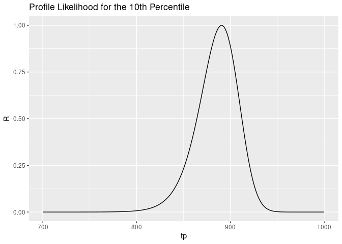
The shape of this curve is as follows:
data.frame(
  tp = seq(700, 1000, length.out = 200)
) %>%
  rowwise() %>%
  mutate(R = profile_likelihood_normal(
    tp,
    0.1,
    c(dat$strength_observed, dat$strength_observed),
    c(rep("exact", 20), rep("right", 20))
  )) %>%
  ggplot(aes(x = tp, y = R)) +
  geom_line() +
  ggtitle("Profile Likelihood for the 10th Percentile")
Next, we’ll find the value of \(u\) that satisfies this equation:
fn <- Vectorize(function(tp) {
  profile_likelihood_normal(
    tp,
    0.1,
    c(dat$strength_observed, dat$strength_observed),
    c(rep("exact", 20), rep("right", 20)))
})

denominator <- integrate(
  f = fn,
  lower = 0,
  upper = 1000
)

uniroot(
  function(upper) {
    trial_area <- integrate(
      fn,
      lower = 0,
      upper = upper
    )
    return(trial_area$value / denominator$value - 0.05)
  },
  interval = c(700, 1000)
)
## $root
## [1] 845.7739
##
## $f.root
## [1] -1.8327e-08
##
## $iter
## [1] 10
##
## $init.it
## [1] NA
##
## $estim.prec
## [1] 6.103516e-05
This value of \(846\) is much higher than the value of \(809\) that we found earlier based on the coupon strength. But, this value of \(846\) is a little lower than the B-Basis of \(852\) that was based on the actual strength of all of the inserts installed.
One way to view the differences between these three numbers is as follows. The B-Basis strength is related to the 10-th percentile of the strength. But it is actually a confidence bound on the 10-th percentile. If we have only a little bit of information about the strength, there is a lot of uncertainty about the actual 10-th percentile, so the lower confidence bound is quite low. If we have a lot of information about the strength, the uncertainty is small, so the lower confidence bound is close to the actual 10-th percentile.
When we calculated a B-Basis from the observed coupon strength, we had 20 pieces of information. When we calculated a B-Basis from the actual insert strength, we had 40 pieces of information. When we calculated the B-Basis value considering the censored data, we had 40 pieces of information, but half that information wasn’t as informative as the other half: the exact values provide more information than the censored values.
Citations
- William Meeker, Gerald Hahn, and Luis Escobar. Statistical Intervals: A Guide for Practitioners and Researchers. John Wiley & Sons, 2nd edition edition, Apr 2017. ISBN 978-0-471-68717-7. 1