All materials have some variability in their strength: some pieces of a given material are stronger than others. The design standards for civil aircraft mandate that one must account for this material variability. This is done by setting appropriate material allowables such that either $90\%$ or $99\%$ of the material will have a strength greater than the allowable with $95\%$ confidence. These values are referred to as B-Basis and A-Basis values, respectively. In the language of statistics, they are lower tolerance bounds on the material strength.

When you’re designing an aircraft part, one of the first steps is to determine the allowables to which you’ll compare the stress when determining the margin of safety. For many metals, A- or B-Basis values are published, and the designer will use those published values as the allowable. However, when it comes to composite materials, it is often up to the designer to determine the A- or B-Basis value themselves.

The most common way of calculating Basis values is to use the statistical methods published in Volume 1 of CMH-17 and implemented in the R package cmstatr (among other implementations). These methods area based on frequentest inference.

For example, if the data is assumed to be normally distributed, with this frequentest approach, you would calculate the B-Basis value using the non-central t-distribution (see, for example,  Krishnamoorthy and Mathew (2008) ).

However, the frequentest approach is not the only way to calculate Basis values: a likelihood-based approach can be used as well. The book Statistical Intervals by Meeker et al. (2017) discusses this approach, among other topics.

The basic idea of a likelihood-based inference is that you can observe some data (by doing mechanical tests, or whatever), but you don’t yet know the population parameters, such as the mean and the variance. But, you can say that some possible values of the population parameters are more likely than others. For example, if you perform 18 tension tests of a material and the results are all around 100, the likelihood that the population mean is 100 is pretty high, but the likelihood that the population mean is 50 is really low. You can define a mathematical function to quantify this likelihood: this is called the likelihood function.

If you just need a point-estimate of the population parameters, you can find the highest value of this likelihood function: this is called the maximum likelihood estimate. If you need to find an interval or a bound (for example, the B-Basis, which is a lower tolerance bound), you can plot this likelihood function versus the population parameters and use this distribution of likelihood to determine a range of population parameters that are “sufficiently likely” to be within the interval.

The likelihood-based approach to calculating Basis values is more computationally expensive, but it allows you to deal with data that is left- or right-censored, and you can use the same computational algorithm for a wide variety of location-scale distributions. I’m planning on writing about calculating Basis values for censored data soon.

Example Data

For the purpose of this blog post, we’ll look at some data that is included in the cmstatr package. We’ll use this data to calculate a B-Basis value using the more traditional frequentest approach, then using a likelihood-based approach.

We’ll start by loading several R packages that we’ll need:

library(cmstatr)
library(tidyverse)
library(stats4)

Next, we’ll get the data that we’re going to use. We’ll use the “warp tension” data from the carbon.fabric.2 data set that comes with cmstatr. We’ll consider only the RTD environmental condition.

carbon.fabric.2 %>%
  filter(test == "WT" & condition == "RTD")

##    test condition batch panel thickness nplies strength modulus failure_mode
## 1    WT       RTD     A     1     0.113     14  129.224   8.733          LAB
## 2    WT       RTD     A     1     0.112     14  144.702   8.934      LAT,LWB
## 3    WT       RTD     A     1     0.113     14  137.194   8.896          LAB
## 4    WT       RTD     A     1     0.113     14  139.728   8.835      LAT,LWB
## 5    WT       RTD     A     2     0.113     14  127.286   9.220          LAB
## 6    WT       RTD     A     2     0.111     14  129.261   9.463          LAT
## 7    WT       RTD     A     2     0.112     14  130.031   9.348          LAB
## 8    WT       RTD     B     1     0.111     14  140.038   9.244      LAT,LGM
## 9    WT       RTD     B     1     0.111     14  132.880   9.267          LWT
## 10   WT       RTD     B     1     0.113     14  132.104   9.198          LAT
## 11   WT       RTD     B     2     0.114     14  137.618   9.179      LAT,LAB
## 12   WT       RTD     B     2     0.113     14  139.217   9.123          LAB
## 13   WT       RTD     B     2     0.113     14  134.912   9.116          LAT
## 14   WT       RTD     B     2     0.111     14  141.558   9.434    LAB / LAT
## 15   WT       RTD     C     1     0.108     14  150.242   9.451          LAB
## 16   WT       RTD     C     1     0.109     14  147.053   9.391          LGM
## 17   WT       RTD     C     1     0.111     14  145.001   9.318      LAT,LWB
## 18   WT       RTD     C     1     0.113     14  135.686   8.991    LAT / LAB
## 19   WT       RTD     C     1     0.112     14  136.075   9.221          LAB
## 20   WT       RTD     C     2     0.114     14  143.738   8.803      LAT,LGM
## 21   WT       RTD     C     2     0.113     14  143.715   8.893      LAT,LAB
## 22   WT       RTD     C     2     0.113     14  147.981   8.974      LGM,LWB
## 23   WT       RTD     C     2     0.112     14  148.418   9.118      LAT,LWB
## 24   WT       RTD     C     2     0.113     14  135.435   9.217      LAT/LAB
## 25   WT       RTD     C     2     0.113     14  146.285   8.920      LWT/LWB
## 26   WT       RTD     C     2     0.111     14  139.078   9.015          LAT
## 27   WT       RTD     C     2     0.112     14  146.825   9.036      LAT/LWT
## 28   WT       RTD     C     2     0.110     14  148.235   9.336      LWB/LAB

We really care only about the strength vector from this data, so we’ll save that vectory by itself in a variable for easy access later.

dat <- (carbon.fabric.2 %>%
          filter(test == "WT" & condition == "RTD"))[["strength"]]
dat

##  [1] 129.224 144.702 137.194 139.728 127.286 129.261 130.031 140.038 132.880
## [10] 132.104 137.618 139.217 134.912 141.558 150.242 147.053 145.001 135.686
## [19] 136.075 143.738 143.715 147.981 148.418 135.435 146.285 139.078 146.825
## [28] 148.235

Frequentest B-Basis

We can use the cmstatr package to calculate the B-Basis value from this example data. We’re going to assume that the data follows a normal distribution throughout this blog post.

basis_normal(x = dat, p = 0.9, conf = 0.95)

## 
## Call:
## basis_normal(x = dat, p = 0.9, conf = 0.95)
## 
## Distribution:  Normal    ( n = 28 )
## B-Basis:   ( p = 0.9 , conf = 0.95 )
## 127.5415

So using this approach, we get a B-Basis value of $127.54$.

Likelihood-Based B-Basis

The first step in implementing a likelihood-based approach is to define a likelihood function. This function is the product of the probability density function (PDF) at each observation ($X_i$), given a set of population parameters ($\theta$) (see  Wasserman (2004) ).

$$ \mathcal{L}\left(\theta\right) = \prod_{i=1}^{n} f\left(X_i;\,\theta\right) $$

We’ll actually implement a log-likelihood function in R because taking a log-transform avoids some numerical issues. This log-likelihood function will take three arguments: the two parameters of the distribution (mu and sigma) and a vector of the data.

log_likelihood_normal <- function(mu, sig, x) {
  suppressWarnings(
    sum(
      dnorm(x, mean = mu, sd = sig, log = TRUE)
    )
  )
}

We can use this log-likelihood function to find the maximum-likelihood estimates (MLE) of the population parameters using the stats4::mle() function. This function takes the negative log-likelihood function and a starting guess for the parameters.

mle(
  function(mu, sig) {
    -log_likelihood_normal(mu, sig, dat)
  },
  start = c(130, 6.5)
)

## 
## Call:
## mle(minuslogl = function(mu, sig) {
##     -log_likelihood_normal(mu, sig, dat)
## }, start = c(130, 6.5))
## 
## Coefficients:
##         mu        sig 
## 139.626036   6.594905

We will be denoting these maximum likelihood estimates as $\hat\mu$ and $\hat\sigma$. They match the sample mean and sample standard deviation within a reasonable tolerance, but are not exactly equal.

mean(dat)

## [1] 139.6257

sd(dat)

## [1] 6.716047

The relative likelihood is the ratio between the value of the likelihood function evaluated at a given set of parameters to the value of the likelihood function evaluated at the MLE of the parameters. The relative likelihood would then be a function with two arguments: one for each of the parameters $\mu$ and $\sigma$. To reduce the number of arguments, Meeker et al. (2017) use a profile likelihood function instead. This the same as the likelihood ratio, but it is maximized with respect to $\sigma$, as defined below:

$$ R\left(\mu\right) = \max_\sigma \left[\frac{\mathcal{L}\left(\mu, \sigma\right)}{\mathcal{L}\left(\hat\mu, \hat\sigma\right)}\right] $$

When we’re trying to calculate a Basis value, we don’t really care about the mean as a population parameter. Instead, we care about a particular proportion of the population. Since a normal distribution (or other location-scale distributions) are uniquely defined by two parameters, Meeker et al. (2017) note that you can use two alternate parameters instead. In our case, we’ll keep $\sigma$ as one of the parameters, but we’ll use $t_p$ as the other instead. Here, $t_p$ is the value that the proportion $p$ of the population falls below. For example, $t_{0.1}$ would represent the 10-th percentile of the population.

We can convert between $\mu$ and $t_p$ as follows:

$$ \mu = t_p - \sigma \Phi^{-1}\left(p\right) $$

Given this re-parameterization, we can implement the profile likelihood function as follows:

profile_likelihood_normal <- function(tp, p, x) {
  m <- mle(
    function(mu, sig) {
      -log_likelihood_normal(mu, sig, x)
    },
    start = c(130, 6.5)
  )
  mu_hat <- m@coef[1]
  sig_hat <- m@coef[2]
  ll_hat <- log_likelihood_normal(mu_hat, sig_hat, x)

  optimise(
    function(sig) {
      exp(
        log_likelihood_normal(
          mu = tp - sig * qnorm(p),
          sig = sig,
          x = x
        ) - ll_hat
      )
    },
    interval = c(0, sig_hat * 5),
    maximum = TRUE
  )$objective
}

We can visualize the profile likelihood function:

data.frame(
  tp = seq(120, 140, length.out = 200)
) %>%
  rowwise() %>%
  mutate(R = profile_likelihood_normal(tp, 0.1, dat)) %>%
  ggplot(aes(x = tp, y = R)) +
  geom_line() +
  ggtitle("Profile Likelihood for the 10th Percentile")

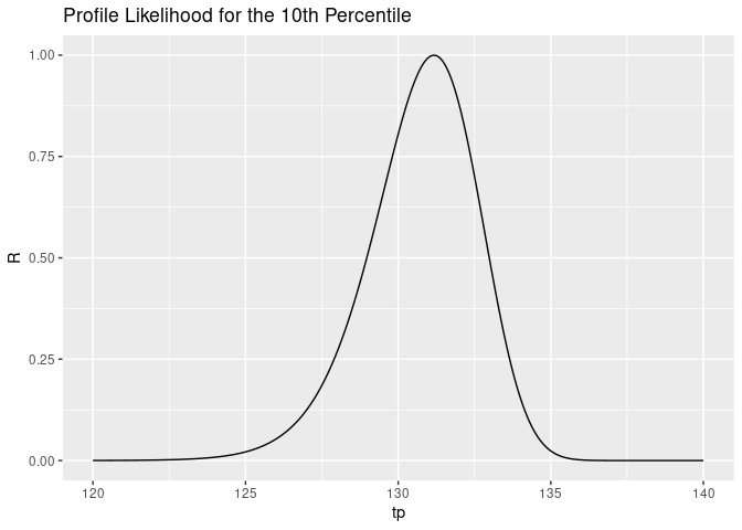
The way to interpret this plot is that it’s quite unlikely that the true value of $t_p$ is 120, and it’s unlikely that it’s 140, but it’s pretty likely that it’s around 131.

However, when we’re calculating Basis values, we aren’t trying to find the most likely value of $t_p$: we’re trying to find a lower bound of the value of $t_p$.

The asymptotic distribution of $R$ is the $\chi^2$ distribution. If you’re working with large samples, you can use this fact to determine the lower bound of $t_p$. However, for the sample sizes that are typically used for composite material testing, the actual distribution of $R$ is far enough from a $\chi^2$ distribution, that you can’t actually do this.

Instead, we can use numerical integration to find the lower tolerance bound. We can find a value of $t_p$, which we’ll call $u$, where $0.05\%$ of the area under the $R$ curve is to its left. This will give the $95\%$ lower confidence bound on the population parameter. This can be written as follows. We’ll use numerical root finding to solve this expression for $u$.

$$ 0.05 = \frac{ \int_{-\infty}^{u}R(t_p) d t_p }{ \int_{-\infty}^{\infty}R(t_p) d t_p } $$

Since the value of $R$ vanishes as we move far from about 130, we won’t actually integrate from $-\infty$ to $\infty$, but rather integrate between two values are are relatively far from the peak of the $R$ curve.

We can implement this in the R language as follows. First, we’ll find the value of the denominator.

fn <- Vectorize(function(tp) {
  profile_likelihood_normal(tp, 0.1, dat)
})

denominator <- integrate(
  f = fn,
  lower = 100,
  upper = 150
)
denominator

## 4.339919 with absolute error < 8.9e-07

uniroot(
  function(upper) {
    trial_area <- integrate(
      fn,
      lower = 0,
      upper = upper
    )
    return(trial_area$value / denominator$value - 0.05)
  },
  interval = c(100, 150)
)

## $root
## [1] 127.4914
## 
## $f.root
## [1] -3.810654e-08
## 
## $iter
## [1] 14
## 
## $init.it
## [1] NA
## 
## $estim.prec
## [1] 6.103516e-05

The B-Basis value that we get using this approach is $127.49$. This is quite close to $127.54$, which was the value that we got using the frequentest approach.

In a simple case like this data set, it wouldn’t be worth the extra effort of using a likelihood-based approach to calculating the Basis value, but we have demonstrated that this approach does work.

In a later blog post, we’ll explore a case where it is worth the extra effort. (Edit: that post is here)